Here is a link to the free Habit Tracker, to make your own copy simply click "File" > "Make a copy". It has been built to help you track up to 15 habits at a time. When you mark a habit completed the line chart will also update to show you a holistic view of how you're keeping up with your habits.
You can make a copy of the template and get started right away but it’s worth understanding how the sheet works so that you can modify it slightly to tailor it to your needs. I'm going to show you how to build a habit tracker that will enable you to monitor whether you’re keeping up with your good intentions. There is a graph at the top of the sheet that will show you what percentage of your habits you’ve managed to keep up with for a given day and show you how that compares with the rest of the month.
We will also break down habits into four categories, health, finances, spiritual, social. Spiritual habits can be meditation, yoga, or journaling. And social habits can be as simple as calling a friend or going on a coffee catch-up. We will also create a doughnut chart about what type of habit you’re prioritizing. Each month you only have to duplicate the tab with the tracker on it and update the name of the month and the rest of the sheet will automatically update.
The first we’re going to do is open up a new spreadsheet in Google Sheets and go to cell A1. We’re going to create a margin for our template by reducing the size of column A before adding our heading to the first two rows. Go down into cell B1 and type Daily Habit Tracker. We are then going to merge cells B1 all the way up to AN1. Change the font to EB Garamond and increase the font size to 25.
We are now going to add an optional tagline below the sheet title by going to cell B2 and typing “Your Habits will determine your Future”. Similarly, to how we merge the title we’re going to merge cells B2 to AN2, adjust the font to EB Garamond, and the font size to 18. We’re then going to add a background color from A1 to AN2 and for this, we're going to use one for the built-in colors, it’s called light red berry 3, adjust the text color to dark grey 3 and center the text.
We’re next going to merge cells B4 to B6 and enlarge the column slightly. Input the first day of the month that you want the tracker to start on. For this example, we are going to use October 1st 2023. Highlight the cell, go to the format number, custom date, and time at the bottom, and then select the month and year format. We're then going to remove the comma and one of the spaces before clicking apply so now only the month and the year will show.
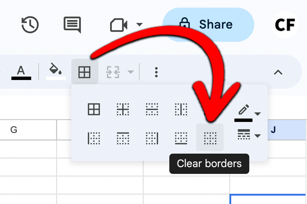
We are then going to match the font color to the color we've been using in the title and center vertically and horizontally and adjust the font size to 21. We're then going to add alter borders but before we do that we're going to add the third option into the dropdown we are then going to change the color to the same color we use in our title. Click apply to alter borders and our sheet is starting to take shape.
We’re next going to add our dates. For this we’re going to use the sequence function, go down to H10 and type equals sequence. For our first parameter, the number of rows was going to enter the number 1. For our second parameter, we’re going to enter 31 because there are 31 days in October. For our third parameter, we’re going to use the date we have in our B4 which in our case is the start of the month, but if you prefer to start on a different date you can enter it in B4. Our final parameter will be 1 because this defines the step increment and we want to track each day.
Above the day of the month we’re going to add the day of the week and to do this we’re going to use the weekday function. So go into cell H9 and type equals weekday H10. adjust the font to EB Garamond and adjust the font color to light red berry 2. We want the day of the week to point up slightly so we’re going to go to text rotation and select tilt up. We can then drag this formula from H9 to AL9 and all of our days will populate.
Next, we’re going to add a few habits to our tracker. You can add your own but I'm going to add meditating, journaling, yoga, call a friend, morning walk, coffee catchup, budget tracker, spend report, finance blog, gym, and a few that we are going to add a placeholder for. We’re then going to go to H11. Then to adjust the color of the checkbox we’re going to go to text color and adjust it to light red berry 3. We can then copy this for the rest of the days of the month and for all of our habits.
We then want to track habit completion. So in cell F27, we’re going to add the word completed. in the row below we’re going to add not completed. And the row below we’re going to add the percentage completed. Now, we want to automatically calculate the percentage completed so in cell H27 we’re going to write equals countif H11 to H26, comma, TRUE. What this does is it looks at our range of habits and if we tick the checkbox it will add it to our total of our completed habit. Checkboxes have two states TRUE or FALSE, we’re TRUE is ticked and unticked is FALSE. This makes them easy to work with when using formulas.
Now for the number of not completed habits we’re going to use the same formula again at this time our criteria is going to be FALSE because we want to add up the boxes that have not been checked. And finally, for our percentage completed row we’re going to divide the total number of completed habit by the total number of habits, and in our case we will write equals H27 divided by H27 plus H28 in brackets. We can then drag these three new formulae from color H all the way along to column AL. Let’s check that our formulas update by checking a few of the boxes in our habit tracker and as we can see the formulae are updating so we know it’s counting correctly.
Now that we have tracked our habit completing percentage we can visualize it on a line graph. To do this we’re going to highlight our percentage completed row go to insert chart and select the smooth line chart. We’re then going to the customized chart in the editor, go down to series, and change the line color to light red berry 2. Next, we need to adjust the line chart and put it where we want it to show, it will also update as we tick off completed habits.
We’re next going to add a divider between our line chart and the checkboxes. To do this we’re going to highlight from A8 to AM8. To borders select the light red berry 3 color and check that we still have the third option selected for the thickness before adding a bottom border. We’re going to do the same on the B10 to B30 except this time we’re going to add a right border.
Everything is starting to take shape now. But the final thing we're going to add is a monthly overview of our habit type. This will allow us to track the type of habits we’re building over the course of the month. we’re going to create a separate tab called habit types and then add a few habit for different types of habits. For this example, we’re going to use spiritual, health, finance, and social. So on the right-hand side of our habit type, we’re going to add a summary table that shows the total number of each type of habit.
Next, go back into the tracker template and go to Insert Chart and under chart type, select donut chart, then under data range delete the current data range and click on the select data range option in the right hand side of the panel. We then going to highlight our summary table on the habit types tab. Now we need to remove the data labels.
The pie graph we’re going to add to our habit tracker is to look at how many tasks we’ve completed versus not completed throughout the month. In cell AM27 we’re going to sum the number of completed tasks and do the same in cell AM28 for not completed tasks. we’re then going to highlight both of those cells and go to insert chart and select the column chart, chart type. After adjusting the colors we are then able to visualize the number of incomplete tasks going down and complete tasks going up as we progress through the month.
So there it is. That’s one way of creating a habit tracker in Google Sheets. It’s the type I use to track new habits and try to add new ones to my schedule as other habits become part of my daily routine. But what works for me may not work for you. The good thing about Google Sheets is that everything we have done today is customizable. So if you don't like the color scheme and layout that we’ve used you can change it to one that you do like.