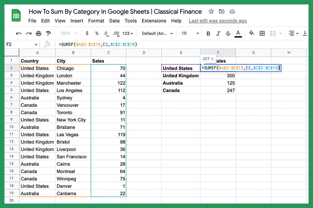
The SUMIF function allows you to specify a range of cells to sum, and a criteria for which cells to include in the sum. Take the example above where you have a spreadsheet with data on sales in the US, UK, Australia and Canada, and you want to find the total sales for each region.
If you would like to take a closer look at the examples, here is the link to the sheet. To edit the data you will first have to go to "File" > "Make a copy".
1) The SUMIF Method
To calculate the category totals you can use the SUMIF function like this:
=SUMIF($A$2:$C$19,E2,$C$2:$C$19)
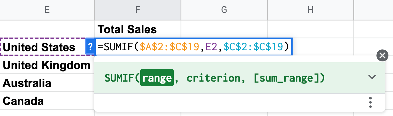
The first parameter is the range, and in our case, it is A2 to C19. We have specified this is an absolute cell reference by using the $ symbol so that we can drag the formula to calculate the sum of the other regions.
The second parameter is the criterion we are looking for, which in this example is the country name.
The third is the sum_range which is the values to be summed if the criteria we are looking for matches.
We can now drag the formula to automatically fill out the sales totals for the other regions. The range and sum range stay fixed because we used absolute cell references.
2) The SUMIFS Method
The SUMIFS method works similarly to the SUMIF example but it does provide some additional functionality should we need it.
We will use the same sample data for this example but this time we will be calculating totals within a country by city. To do this we need to match both columns a and b before summing the sales value.
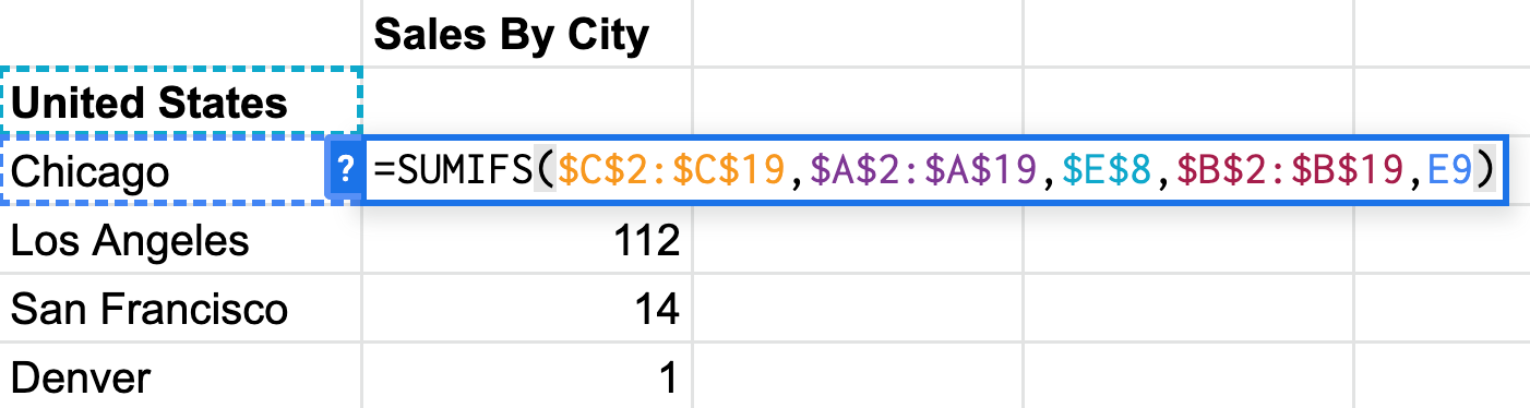
=SUMIFS($C$2:$C$19,$A$2:$A$19,$E$8,$B$2:$B$19,E9)
The SUMIFS function has additional parameters that allow us to match more than one criteria before summing: SUMIFS(sum_range, criteria_range1, criterion1, [criteria_range2, criterion2,...])
In the example, our sum_range is column c (which contains the number of sales), our first criterion is country which needs to be the United States in this example. The second criteria match we are looking for is the city which we look for in column b.
3) The IF + MATCH + SUMIF Method
We can combine multiple functions as another way to sum based on multiple criteria. In this example, we will calculate the total sales by city in the United Kingdom.
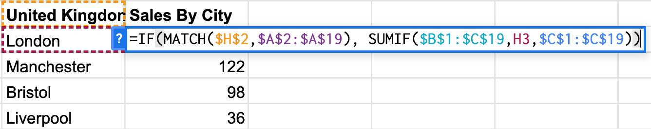
=IF(MATCH($H$2,$A$2:$A$19),SUMIF($B$1:$C$19,H3,$C$1:$C$19))
The MATCH function first checks that we are only looking in the UK, then, if it's true the SUMIF function adds up the sales based on the specific city we are searching for.
Additional Notes
If the same categories appear multiple times in a list it can be helpful to create a new list that groups them. To do this we can use the UNIQUE function.

In our original list, we have a list with 18 countries but they are not unique. To create a list of unique values we can type =UNIQUE(A2:A19), this will return a new list containing only unique values.
The SUMIF function is the simplest way to sum by category in Google Sheets (other than calculating manually if you are trying to avoid functions). However, there are other cases where using SUMIFS or nested functions are necessary. Go with the method that will work best for what you need.
If you have any questions or comments, please let us know!