Check here for the example datasets that we use for the examples so that you can follow along in real time. And if you ever get confused or stuck, you can come back to them to remind yourself of how it all works.
Without further ado, let’s dive straight into the SUM function.
Unlike many other spreadsheet functions, the SUM function is both easy to use and easy to explain - it will calculate the sum of a range of cells for you. This can be rows, columns, or specific cells that you select. You can vary the range however you choose to, and the SUM function will return the total of every cell that you have included.
You can sum huge amounts of data without having to manually input each number which can save you a lot of time. Your data will also update ‘live’, so if you update a number within your SUM range, the totals will automatically update.
This can be particularly helpful when making projections and plans, or setting targets - you can play around with your data to see how varying figures will impact on the overall totals.
No matter how much data you want to use in this formula, there are only a couple of things that you need to remember.
SUM Formula
The formula looks like this:

There are only really two components to it. First we have the =SUM(, this is basically signalling to Google Sheets what function we want to use, which in this case is the SUM function. Then we need to tell the function which cells we want to add up. This could be an entire row, column or a select group of cells. That’s all there is to it.
The best way to understand a formula is to run through some real world examples. So that's what we’re going to do:
#1 Summing Columns
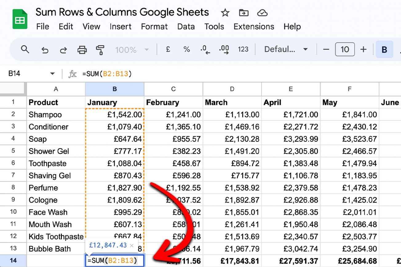
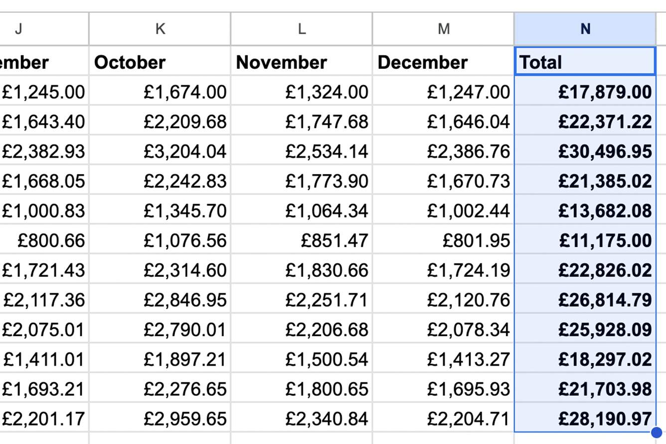
For our first example we are going to look at some data from a fictional toiletry products supplier. They have a spreadsheet with each of their twelve products listed on a separate row in column A. And in row 1 they have the twelve months of the year. The data that they record is the total sales for each product in each month of the year.
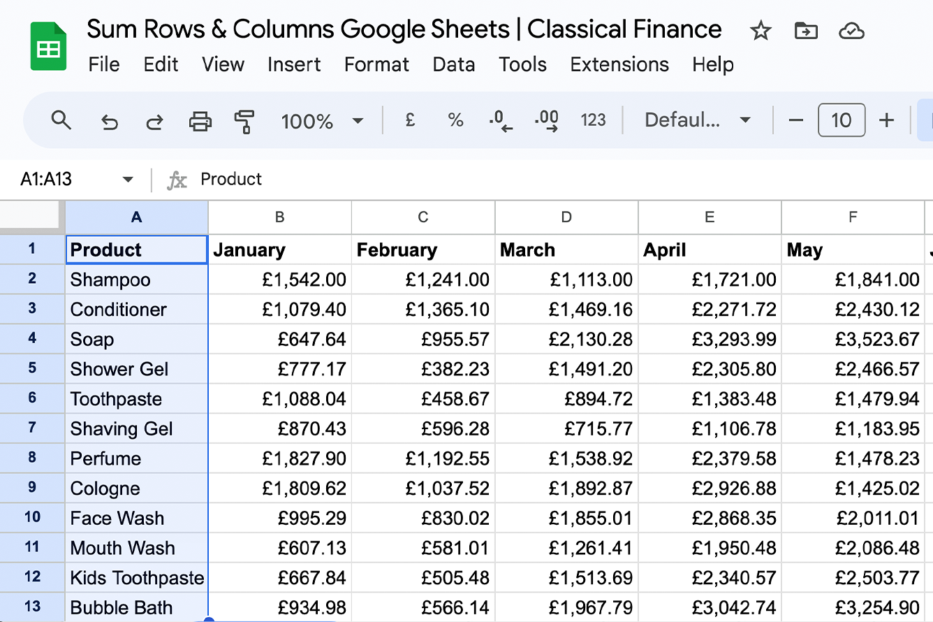
You can probably guess where this is heading! While it’s great to have all of this data in one place, it would be far more helpful if we could have the totals - both for each month of the year, and for each product. So how can we do that?
Well, pretty easily! We can use the SUM function for our rows and our column to generate these totals and have everything there on one sheet. If you would like to follow what we are doing, just go to the ‘Example 1’ tab on the Google Sheet in the link below this video.
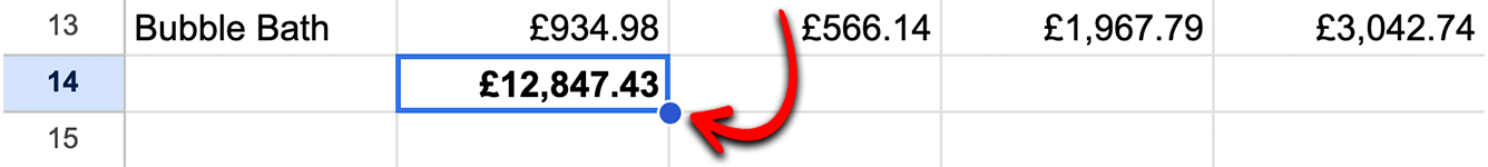
First off, we’ll sum the columns, a total for each month of the year. And naturally we’ll start with January. So let’s head to the cell B14 - in the column underneath the last product row to enter our formula.
We’ll start, as ever, with the equals sign (=), and then write SUM next to it, to let the Sheet know that we would like the total of the cells that we are about to select. Then we will need to open our brackets by holding shift and pressing the number ‘9’ on our keypad. Google Sheets might be ahead of us at this point, and suggest the range that we’ll want to use, but for this example we’re going to ignore that and do it ourselves, just to make sure we understand how it works.
So to enter the range we have two options - we can type in the cells that we want to use, or we can click on them with the mouse and it will be automatically filled into the formula.
If we were to type it in, we would write in the first cell that we want to use, which in this case is cell B2. Then, instead of having to type in every cell that we want to include, we can just type a colon (:) which in this context means ‘every cell up to and including’ and then type in the last cell that we want to include, which in this case is cell B13.

Then we close our brackets (by holding shift and pressing ‘0’) and hit enter. Then our total will appear in the cell - the total amount taken by our company in January.
Now it’s time for another great time-saving feature on Google Sheets. Rather than typing the same formula over and over again for each of the months on the spreadsheet, we can just fill the one that we have just written across to all of the other columns, and it will be automatically adjusted to use the relevant cells for each month.
To do this, we just need to click and hold on the little blue circle in the bottom right of the cell, and then drag it across to the 11 other columns.
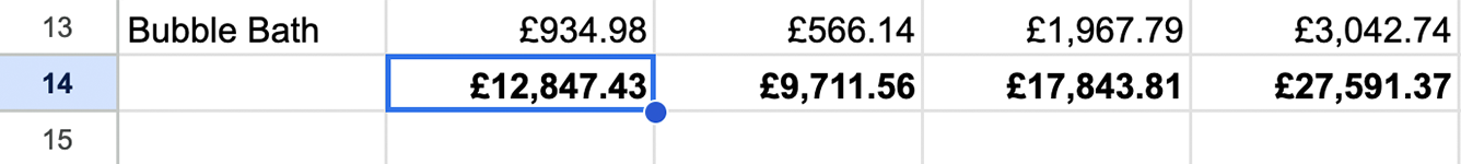
Then you will see the total for each month displayed in row 14, all the way across. It’s as easy as that.
#2 Summing Rows
We covered how to sum columns but what if we want to sum rows too, and how would we sum only certain values from each row? In this example we are going to find the total sales for each product over the whole year - and to get this we will need to add up each month. Fortunately, we now know how to do this!
In the last example, I said that there were two ways to enter the cell range, one by typing, one by using the mouse, so for this example, we will use the mouse so that you can get comfortable using both methods. Don’t worry though, this is just as easy, if not easier.
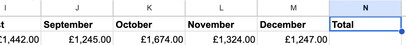
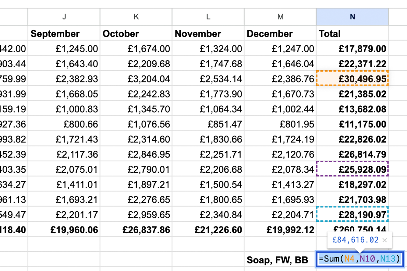
So let’s add in an extra column to the right of our data, which we’ll give the heading ‘Total’.
Then in the first row of data, row 2, we’ll add in our formula. So let’s go to cell N2, and make a start.
We’ll first type in the equals sign, and then write the word SUM as we did before, before opening up the brackets. Now, to enter the cells that we want to include, rather than typing them out let’s click on them. Not only can this be easier, but you are also less likely to make a mistake - typos when writing formulas are a frequent cause of errors and this more visual method can help you avoid them.
So, with the brackets open, we can first click and hold on the first cell, which just so happens to be cell B2 again, and then drag that all the way along the row to the final cell that we want to include, which is cell M2. You will see now that the text B2:M2 has been automatically filled into our formula, so all we need to do is hit enter and our total figure for Shampoo sales is entered into cell N2.

And now we know how to fill this formula into all of the other rows - we’ll just click and hold onto the small blue circle in the bottom right of the cell again, and drag it all the way down to cell N14 - this will then include the monthly totals that we made in the first example, and therefore giving us the overall sales figure for that year.
And there we go, we have now used the Sum function on our column and rows to give us totals.
What if the data I want to total isn’t all in one place?
There is one final thing that you might need to consider when using the SUM function - what if you want a total for just a few sections of a column or row, that doesn’t run in one complete block. To use an example from the data we have been using, what if you would like a quick year total for just a few of the products? Say, Soap, Face Wash and Bubble Bath?
Well, we just need to alter the way we select our range - everything else stays the same. We still start off with =SUM and open our brackets. But then we need to select just the cells that include the data we need - so in this case it would be N4, N10 and N13.

If we are typing in our range, we will type in each cell, separating them with a comma - so (N4, N10, N13), and hit enter. If we are using our mouse, we will hold down control and click on the three cells, which will automatically fill them into the formula, just like before.
Then we hit enter, and hey presto - we have our total for that specific group.
Conclusion
Thank you for reading this guide, we hope that you have found it helpful. As we said at the start of the article, the SUM function is the most used on Google Sheets, so it is so important that you are comfortable and confident using it. It’s the first step to really making the most of what Google Sheets has to offer.
If you have any comments for us, or if you have any requests as to what we can cover in future articles, please leave them in the section below - we would love to hear from you.