Working with Google Sheets often requires data imports from other sheets. IMPORTRANGE is a helpful function enabling you to work across multiple sheets and share data between them. If you would like to try the examples for yourself, open the Google Sheets links, select "File" from the toolbar and select "Make a copy".
IMPORTRANGE Formula
The IMPORTRANGE function has two required inputs, the spreadsheet_url and range_string.

- The spreadsheet_url specifies the URL of the spreadsheet you intend to import data from. It must be enclosed within quotation marks or otherwise be a reference to another cell containing the spreadsheet URL.
- The range_string parameter selects the data to be imported. Range_string is composed of two elements, the sheet name and the range within that sheet to be imported. It is formatted as the sheet name, followed by an exclamation mark, followed by the range, for example, "Sheet2!A1:B10".


- Either the full URL or just the spreadsheet ID can be used for the spreadsheet_url parameter.
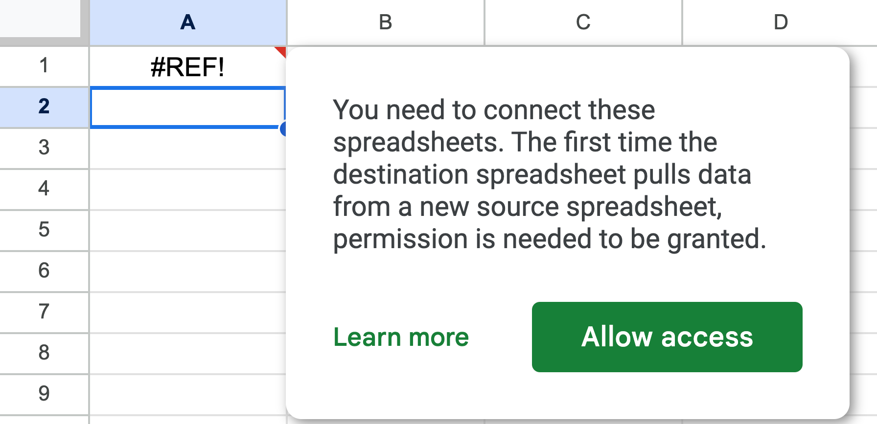
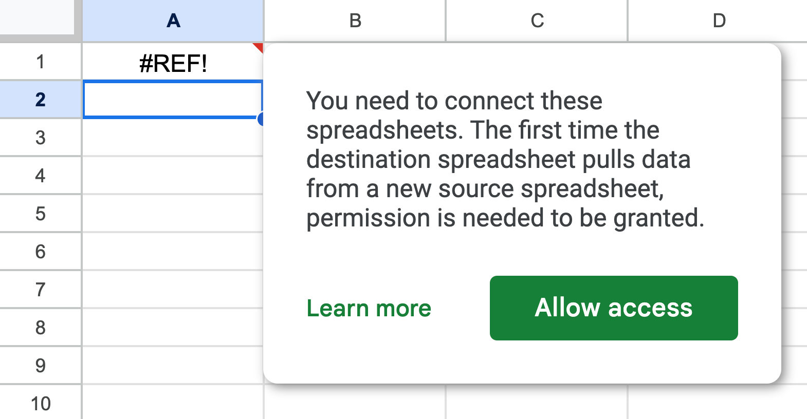
- The first time you try to import from another sheet you will see a #REF! error. You will need to press "Allow access".
- If you do not own the spreadsheet you are trying to import data from you will receive the error, "You don't have permissions to access that spreadsheet". If this happens you can go to the URL of the spreadsheet and request access. If the owner grants you access as an editor you will be able to import data using the IMPORTRANGE function.
IMPORTRANGE will automatically check for updates every hour while the sheet is open to ensure the data is up-to-date.
Example #1
In the first example, IMPORTRANGE will be used to import a table from a source spreadsheet to a main spreadsheet. You can access the live source spreadsheet here and the sheet where the IMPORTRANGE function will be used is here.
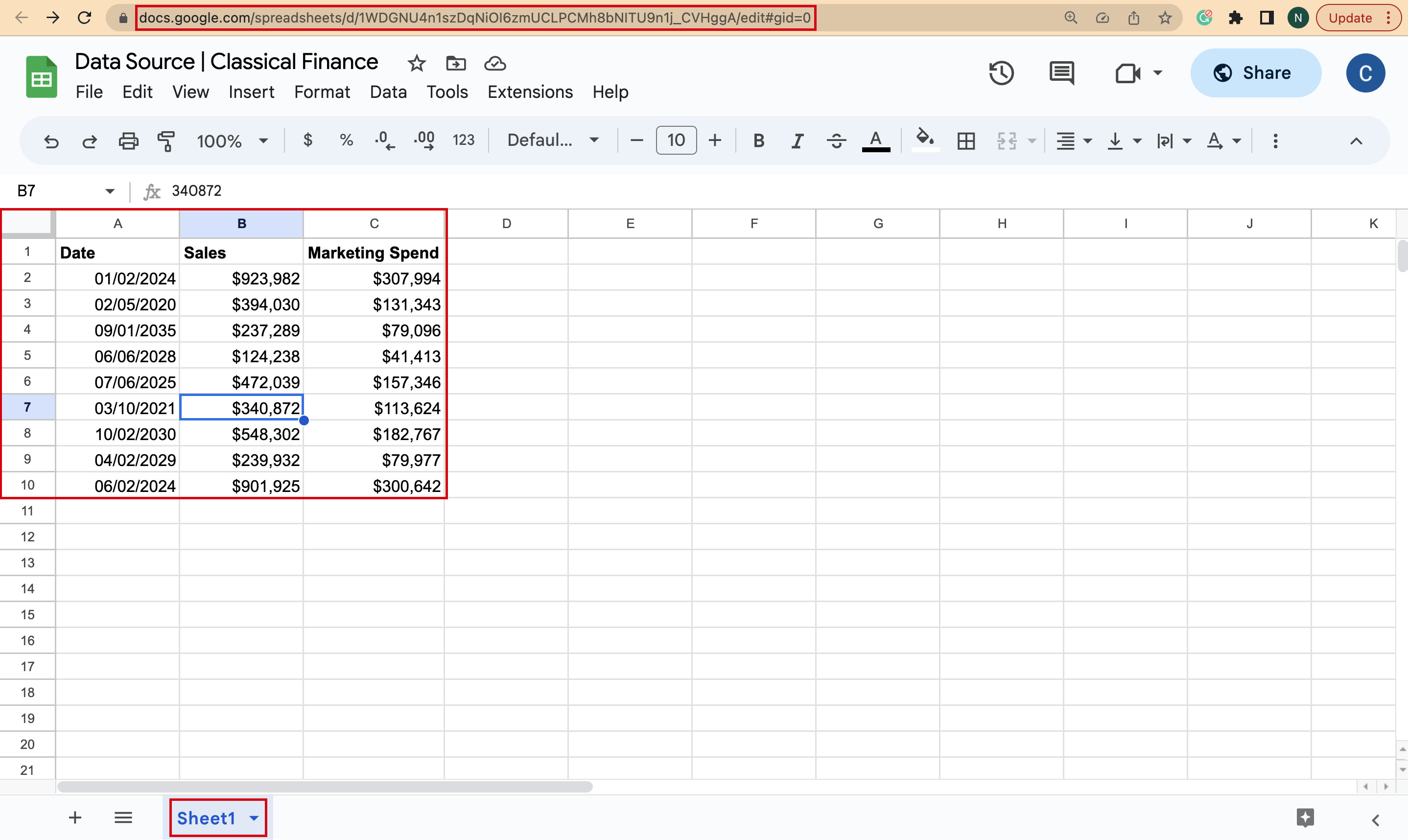
On our source data sheet there are three key pieces of information we need to take a note of in order to correctly format our IMPORTRANGE function:
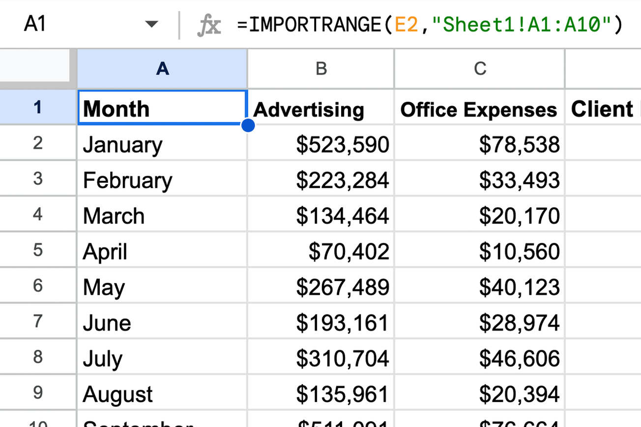
- The URL of the spreadsheet, which is located in the address bar and highlighted below.
- The range of the data, in this case it is A1:C10.
- The name of the tab upon which the data is located, in this case it is "Sheet1".
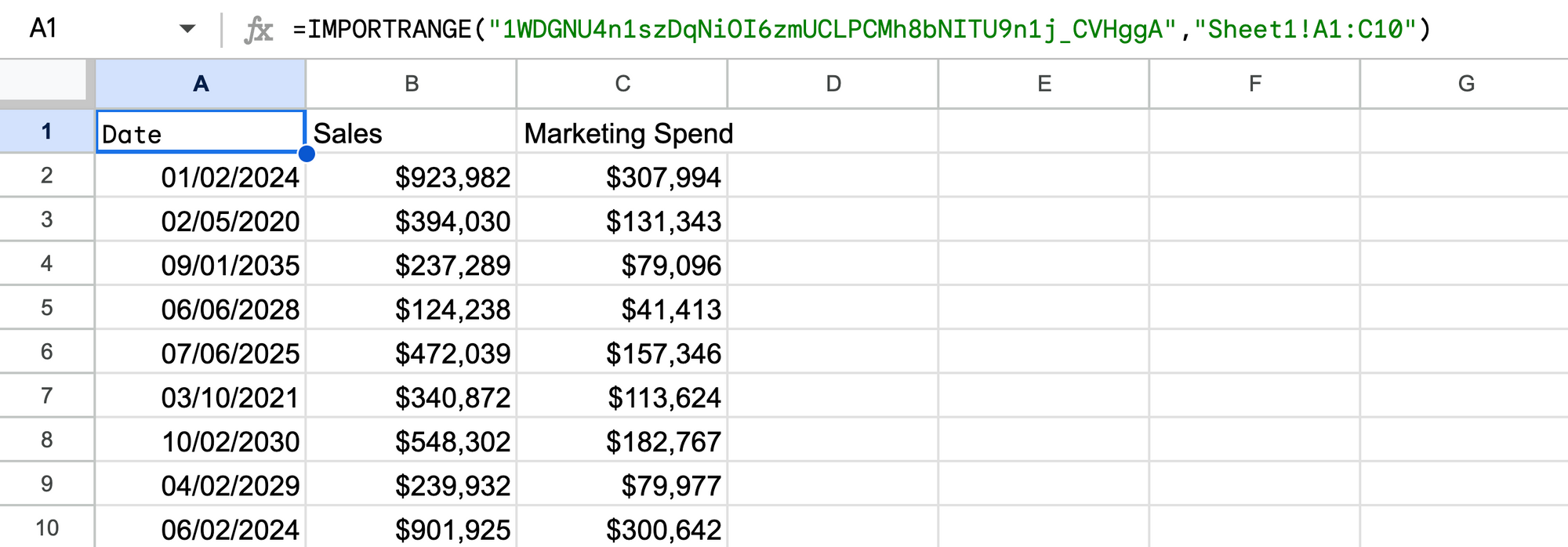
Once we have these parameters we can return to our main spreadsheet to begin writing our IMPORTRANGE function. In this example we will use our spreadsheet ID, which we can use for the spreadsheet_url and our range string Sheet1!A1:C10.
Putting both parameters into the IMPORTRANGE formula we arrive at the function below:

Next, grant permission for the sheet to pull data from the source.

After a short loading period, the date from the source sheet will appear in the main sheet, as shown below. Adjusting the amount of data imported can be achieved by adjusting the range_string cell parameters.
N.B. In the above example we have just one tab on the sheet we are importing from, so by default it is the first (and only) sheet. In this example it is possible to omit the tab name in the range_string parameter. This is because Google Sheets defaults to the first tab when the tab name is left out of the query.

However, when working with data across multiple tabs, it is important to include the sheet name.
Example #2
In many situations, data in the source sheet will need to be filtered and reordered when being imported. In our second example we will look at filtering the imported data using IMPORTRANGE multiple times.
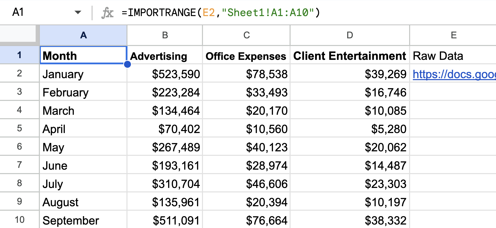
The raw data this time has multiple additional columns.
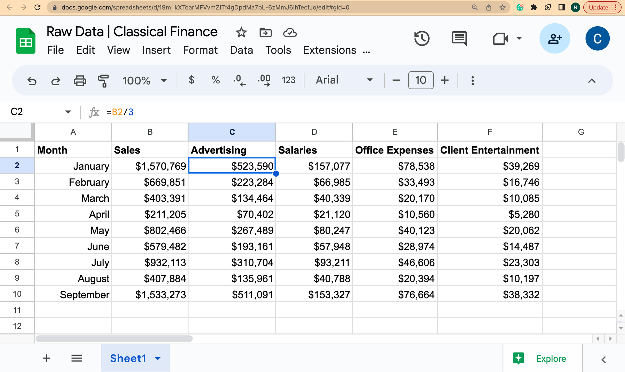
The boss wants to take a closer look at advertising costs, office expenses, and client entertainment each month. He is not familiar with Google Sheets and has asked us to present it on another document.
The first way to achieve this filtered view is via using the IMPORTRANGE function three times which is the method we will demonstrate first. In this example, we will be using the same spreadsheet_url multiple times so instead of using the full URL we will use a cell reference. Our spreadsheet will be in cell E2.

The first time the sheets are connected we will again need to allow the main sheet to access the source sheet.
The data for the month is in column A, advertising costs in column C, office expenses in column E and client entertainment in column F.
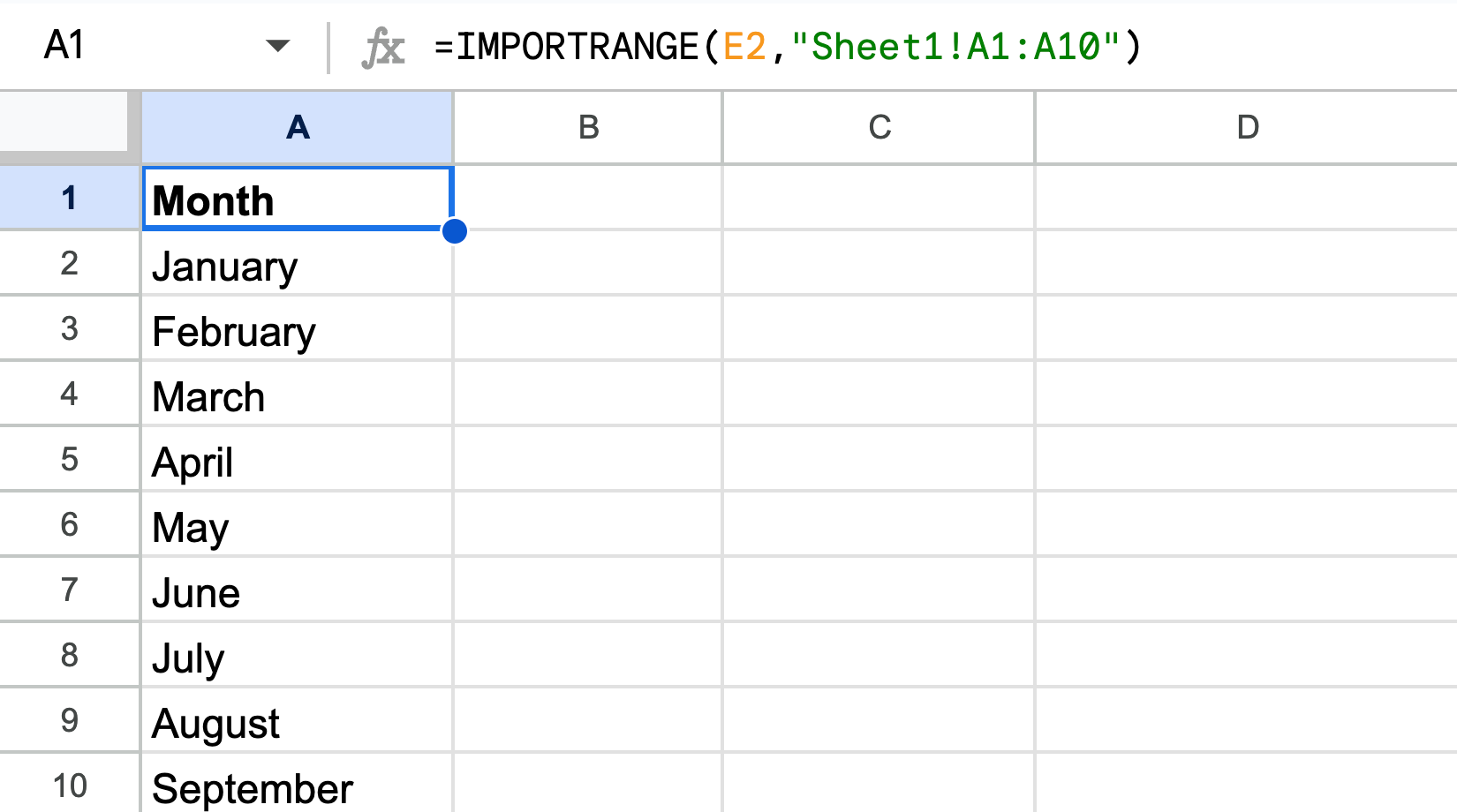
To filter for just the month column, the formula will be:

Filtering for advertising costs will be the same, except we need to adjust the column being imported to column C.

We can combine the import for columns E and F as they are alongside each other in the source sheet.

The result is a filtered table with all of the data we need in the format we needed it in!
Wrapping Up
The intention of this guide was to demonstrate multiple ways in which the IMPORTRANGE function and its parameters can be used. However you need to import your data, I hope this guide has given you a foundational understanding that you can apply to your specific problem. If you have any questions, don't hesitate to drop a comment down below.