Here is how you sum a filtered list in Google Sheets:
- Type =SUBTOTAL( into the cell you wish to display the sum in.
- Use 109 for the first parameter followed by a comma and then input the range of the filtered list e.g. =SUBTOTAL(109, A1:A10)
- Hit enter to reveal the total.
Explanation
The SUBTOTAL function takes a function_code as its first parameter. Entering the number 9 tells Google Sheets to sum the values in the specified range. Then, prepending it with the number 10 lets Google Sheets know to skip the hidden cells. Click here for a working example.
SUBTOTAL Function

The SUBTOTAL function calculates subtotals from vertical lists. Its first parameter, the function_code can be adjusted to change the way it aggregates.
- 1 for AVERAGE
- 2 for COUNT
- 3 for COUNTA
- 4 for MAX
- 5 for MIN
- 6 for PRODUCT
- 7 for STDEV
- 8 for STDEVP
- 9 for SUM
- 10 for VAR
- 11 for VARP
To avoid hidden cells the number 10 is prepended to this function_code. Additional cell ranges can be incorporated by adding them after the initial one e.g. =SUBTOTAL(function_code, range1, range2...).
Notes:
- When an autofilter is applied, the cells filtered out are not included in the SUBTOTAL regardless of the function_code.
- The SUBTOTAL function will also filter our other SUBTOTAL functions within the range specified. This is to prevent double-counting e.g. if the function is being applied to the entirety of column B, and column B already contains SUBTOTAL functions, those cells will not be included in the new SUBTOTAL.
Example #1
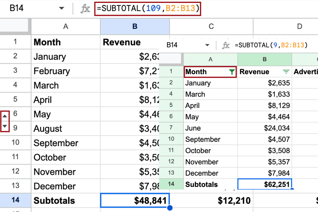
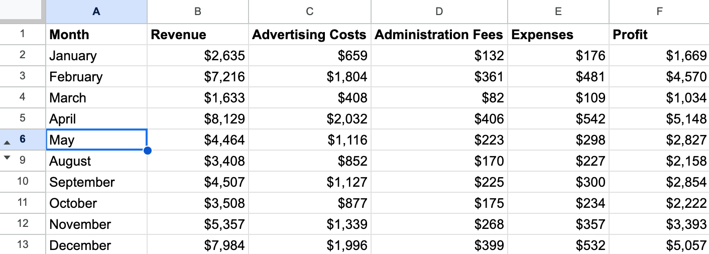
The example here contains the financials for a profitable (but fictional) company. The boss has hidden rows 7 and 8 and wants subtotals calculated in row 14. Now it would be possible in this particular example to do it manually but we're going to use the SUBTOTAL function instead.
To do this we need two parameters, function_code and range. We want the sum so we're going to use 9 and because we want to exclude hidden cells we will prepend it with 10, giving 109. The range for the first subtotal is B2:B13 so we will use that for our second parameter. Combining them together results in the following function: =SUBTOTAL(109, B2:B13).
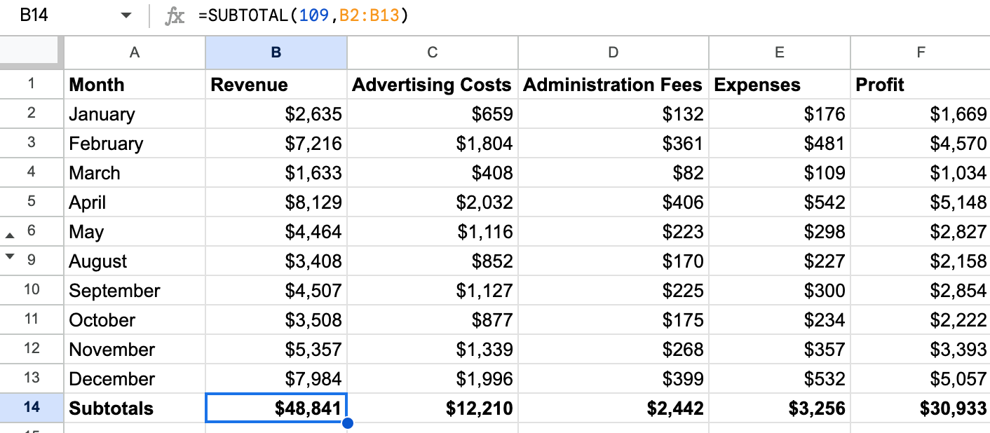
The formula can then be dragged across to column F to calculate the totals for the other subtotals.
Example #2
In the second example, we will look at subtotaling the same table but this time it has been filtered in a different way. The example spreadsheet is here if you would like to follow along.
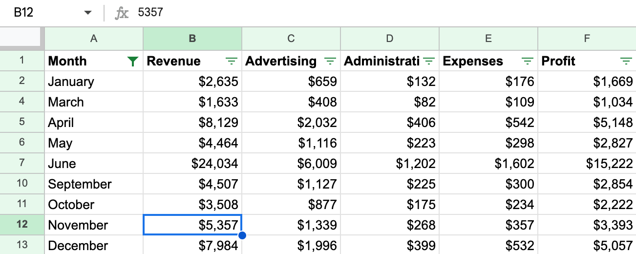
The data has been filtered using the inbuilt autofilter in Google Sheets, and the months of February, July, and August have been removed. This autofilter means the SUBTOTAL function will automatically skip the filtered cells so we don't need to prepend the function_code with 10 this time. So we can proceed with the formula =SUBTOTAL(9, B2:B13).
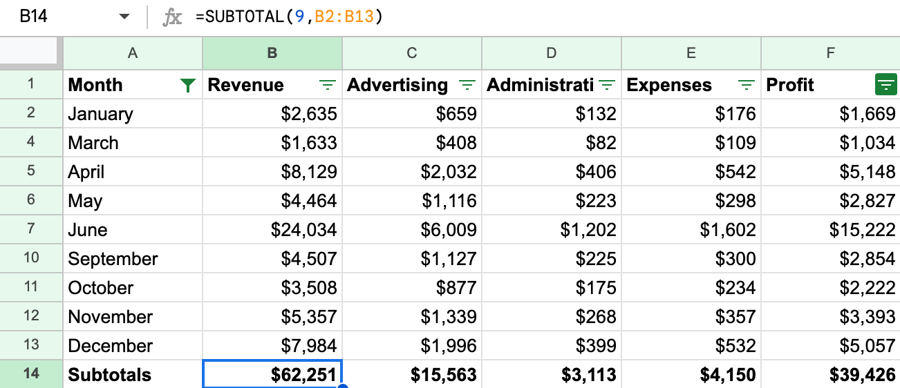
In this case, using the function_code 109 would have given the same result but it is worth noting why it can be omitted in this case.
The above explanation should cover the majority of use cases for subtotaling filtered data. If there is a concept that has not been covered that you are struggling with and would like help, leave a comment down below and we'll do our best to get back to you.