The SUMIF function in Google Sheets is an enhancement of the basic SUM function. SUMIF calculates the ‘SUM’ of values in a range based on ‘IF’ they meet a specified condition, which is referred to as a ‘criterion.’
-
Example 1: Sum Of Positive Numbers
Example 2: Date Criteria
Example 3: Text Condition
Common criterion examples are if a number is greater than (>), smaller than (<), or equal to (=) another number. Once a criterion has been established, the SUMIF function calculates the sum of the data points that meet the condition.
SUMIF Formula
The syntax of the SUMIF function is as follows:

SUMIF has three variables:
- Range (required): the range of cells that are to be evaluated by the criterion.
- Criterion (required): the specified condition to be met within the range. The criterion can be a number, date, text, cell reference, logical expression, or any function.
- Sum_range (optional): is an additional step for specifying a range in which to sum numbers. If you skip this step, the range used by the criterion will be calculated instead.
The SUMIF function is used in the same way in Microsoft Excel. If you’re looking to transfer files between the two programs, you do not need to worry about making edits when exporting this function from Google Sheets to Excel and vice versa.
Example 1: Sum Of Positive Numbers
Numeric conditions will calculate the sum of the numbers that fit within your range and criterion. Such a criterion can be whether a number is greater than (>), less than (<), and/or equal to (=) a specified number.
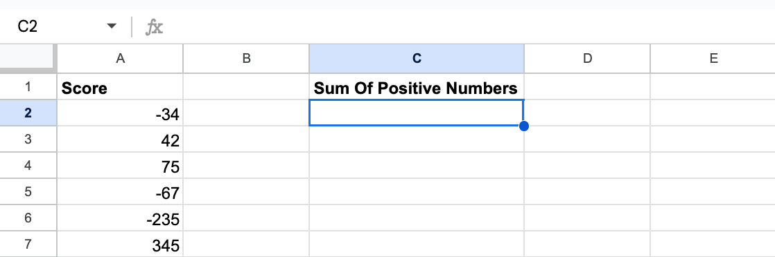
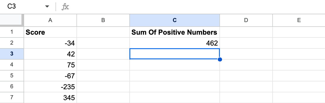
Our first example will take a range of numbers and look to sum the positive numbers.
Step #1:
Select the cell where you will input the formula (C2 in this example).
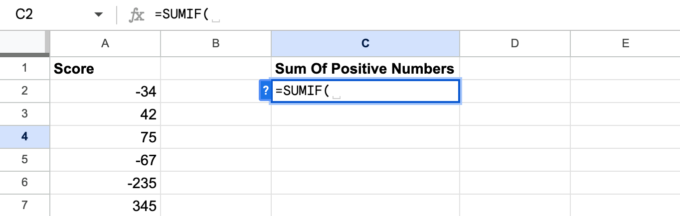
Step #2:
Input the function: =SUMIF(
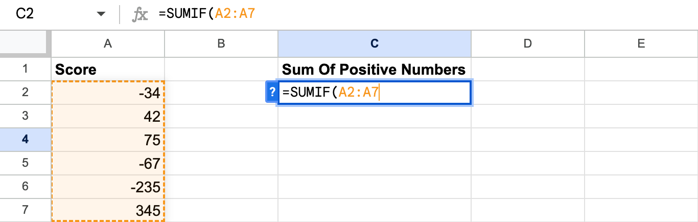
Step #3:
Within the opening bracket, enter the first variable. This information will be the range of data that will be assessed by the SUMIF function in the final calculation. In this instance, it is A2:A7.
Step #4:
The second variable, which is the condition, will specify the numbers that will be calculated within the selected range. In this case, it is ">=0,” meaning the numbers that are greater than (>) or equal to (=) zero will be calculated. This will separate the positive numbers from the negative.
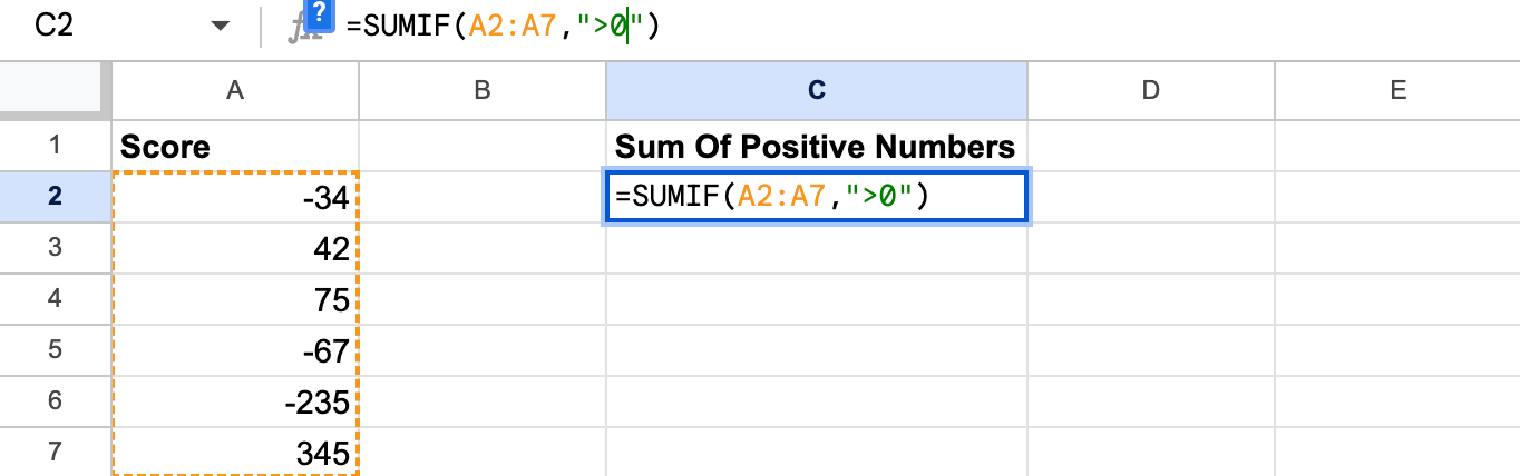
Step #5:
Press Enter to execute the formula and calculate the sum of the positive numbers, in this case, the result is 462.
Example 2: Date Criteria
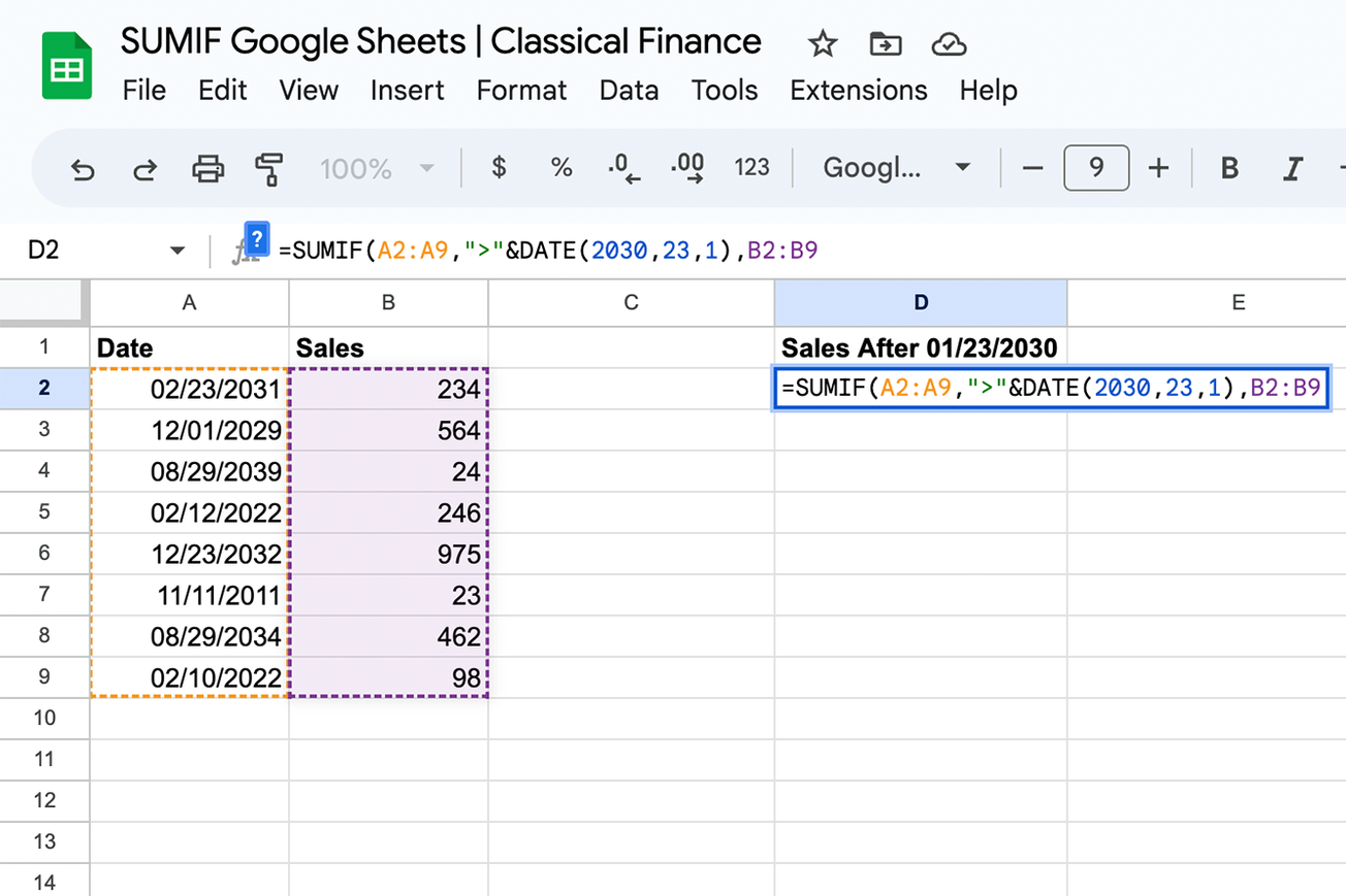
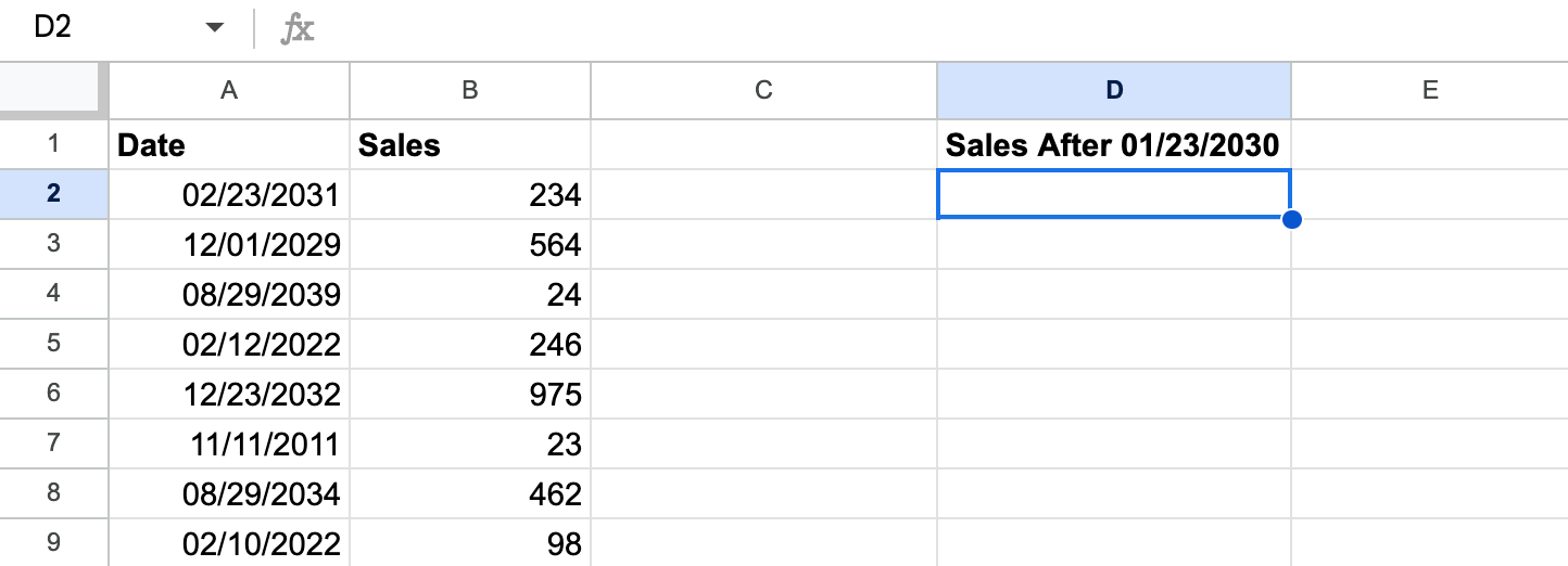
SUMIF allows for date-based criteria too. In this example, we will sum the total number of sales after a given date.
Step #1:
Select the cell where you want to perform the function. In this example we will use D2.
Step #2:
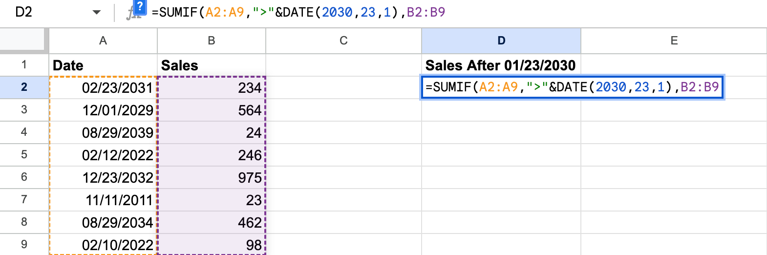
Input the following formula to tell the function to only sum dates after 01/23/2030, =SUMIF(A2:A9,">"&DATE(2030,23,1),B2:B9).
Step #3:
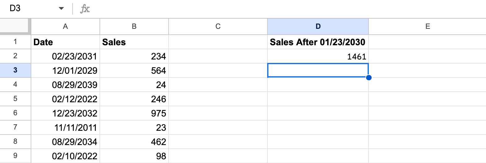
Hit enter and the result will be calculated. In this example, the correct answer is 1461.
Example 3: Text Condition
Text conditions can be used as a criterion to help you calculate a numeric total in relation to a text-based entry.
For example, if you have a list of people or items in one column, and numbers in a neighboring column, you can use specific text as the criterion. You can then add the optional “sum_range” to the formula. If you select the numeric data for this range, the numbers that are assigned to the relevant text will be used to calculate the final sum.
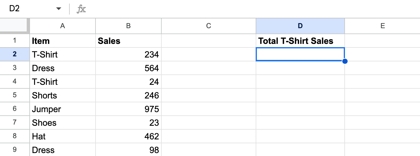
For this example, we will look at look at data for a clothing sale and use SUMIF to determine how many T-Shirts were sold.
Step #1:
Select the cell where you want to input the function (D2 in this example).
Step #2:
Type the following formula in the cell: =SUMIF(A2:A9,"T-Shirt",B2:B9)
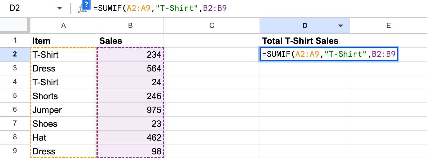
- A2:A9 is the range of the criterion.
- T-Shirt is the text condition.
- B2:B9 is the ‘sum_range’ - the numerical range that will be added together based on the criterion for the total sum.
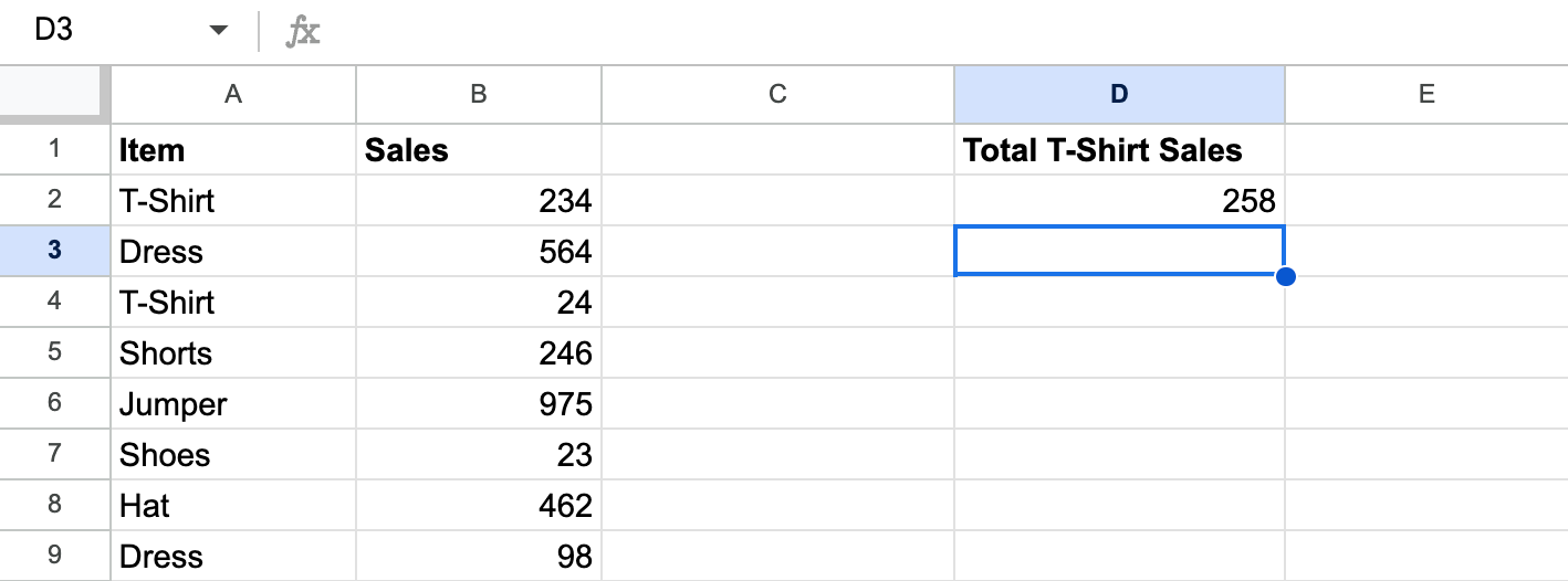
Step #3:
Press the Enter key to complete the formula. We can see that the total number of T-Shirts sold is 258.
SUMIF vs SUMIFS
SUMIF and ‘SUMIFS’ are similar functions: They both sum cells within a range based on whether they meet a specified criterion, but there is a slight difference.
If you want the convenience of SUMIF, but want to further refine your data, you can use SUMIFS for multiple criteria. The SUMIF function is limited to one criterion, while SUMIFS counts cells within a range that meet multiple conditions.
For example, if you have multiple columns of data in your document, you can have a criterion based on text, and then further refine it by adding an additional numerical criterion for the text-based cells to meet.
Why the SUMIF Function is Important in Google Sheets
Learning about Google Sheet’s many functions can transform the way you use it.
One of the greatest benefits of the SUMIF functions is that it can save a massive amount of time, especially when handling a large volume of data. By being able to calculate sums based on specific criteria, you can get various pieces of data within seconds when you have a well-organized document.
The SUMIF function can also help you wrangle an incomprehensible set of data, whether it’s of a large volume, or has a diverse range of entries.
The ability to filter the data so you can get the sum of specific criteria means that you can make sense of a large quantity of data, by simplifying multiple entries into a more condensed format.
Calculate Sums Across Ranges Easily
The SUM function is a basic method of calculating the sum of entire rows and columns, but is not feasible when you want the sum of specific values within a range.
Learning how to use the SUMIF function is essential when handling more advanced data in Google Sheets. The more advanced version of SUM can allow you to come up with totals for specific criteria and ranges, allowing you to understand, present and filter your data better.
How to use the SUMIF Function in Google Sheets
Here, will go through some examples of how you can use the SUMIF function in Google Sheets. There are a number of types of criteria that you can use with SUMIF, and we will cover them here.
To Conclude
We hope this guide has helped you learn the SUMIF function and how to use it in Google Sheets. The SUMIF and SUMIFS functions are valuable assets for anyone working on Google Sheets, and the same rules are often transferable to Microsoft Excel.
While the number of functions and formulas at your disposal may seem intimidating, they’re there to make your data processing experience more straightforward and efficient.
Once you learn the basics of how to use Google Sheets, you will be able to work with a vast amount of data and condense it down to more understandable values within seconds.