First of all we are going to run through what VLOOKUP is used for, and how it might be able to help you, and then we are going to run through a couple of examples so that you can see, step by step, exactly how this function works and how you can apply it to your own data.
You can follow along too. Click on this link to find the datasets that we have used for these examples, meaning you can check back on them at any point if you need a reminder of how it all works.
Classical Finance - Google Sheets Mastery
Learn The Sheets Skills Used By Fortune 500 Companies In 30 Days
Okay, now it’s time to get started.
What is VLOOKUP?
VLOOKUP actually stands for “Vertical Lookup” - it’s a standard function within Google Sheets that scours your spreadsheet vertically to find a specific piece of data. Or to put it in a simpler way, it’s a formula which can find the information you are looking for - it will scan to find the information which can then be cross-referenced or displayed with some other data.
Using VLOOKUP, you can find that information immediately, without having to manually scan through all of the data - so it can save you a lot of time.
It can seem quite a daunting function to use, though, as when you first look at the function it can seem a bit complicated. There is a set syntax that is required for the function to work that you need to understand before you can use it, but it is much simpler than it looks.
Here is the syntax:

Now let’s break that down piece by piece. The first parameter is the Search_key. This refers to the value that you are searching for - so for example, if you were searching for a particular order number, you enter the cell that contains that information here.
After that, we enter the range - this is where we are going to be looking for the data, which will be two or more columns. The first column will always be the place where it looks for your Search_key.
Then we are on to index, which is the column number that we want to extract data from. So, for example, if you wanted the order value of each of the orders that you selected in the Search-key section, and this figure was in the next column, you would enter 2, as the information you want is in the second column.
Finally, we have [is-sorted]. This has to be either True or False, but most of the time it will be False. You would only enter True if the first column in Range is sorted in ascending order - this would return the closest match to your Search_key. If you, as you will in most cases, enter False here, the formula will only look for the exact match from your Search_key.
If you are struggling a little bit to take all that in, don’t worry - it will all start to fall into place now as we run through a couple of examples using our fictional commercial bakery. You can follow exactly what we are doing by clicking on the link in the section below.
Example 1
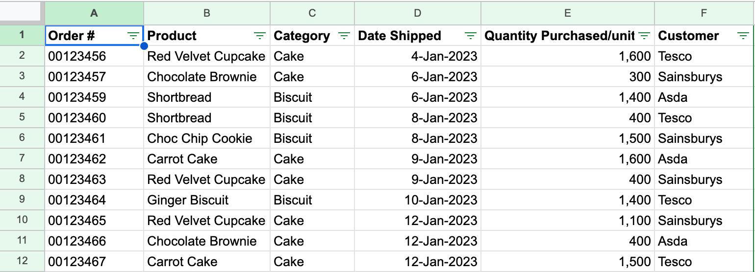
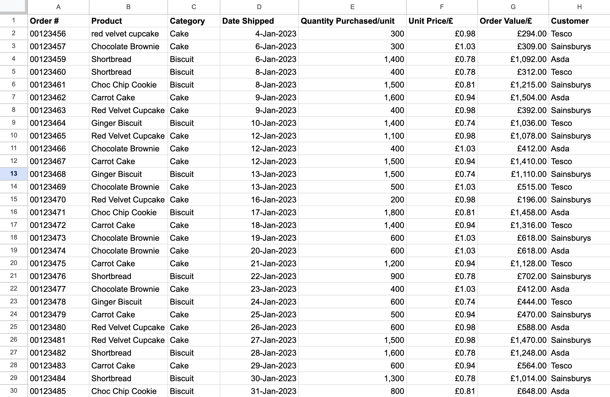
It’s a stressful day in the office of our bakery as one of their customers, Asda, have been in touch to say that they haven’t received a number of orders that they have placed. They have provided a list of order numbers, so our team needs to get to the bottom of it and find out when each of them were shipped, so that they can speak to the, usually reliable, courier company. Here is the data.
Going through the huge list of orders would take too long, so they decide to do a VLOOKUP to get the date that each of these orders were shipped. Let’s help them out.
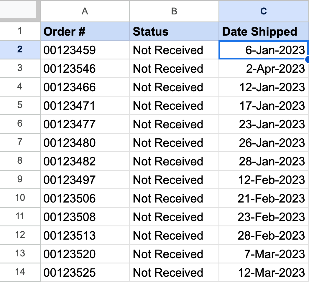
First of all, we are going to create a new sheet, named ‘Missing Orders’, so that we keep all the information in a neat, clear place. VLOOKUP works between different sheets. The first step is to enter each of the orders that our customer has claimed are missing in the first column, and we’ll add a Status column to mark them all as Not Received. Now we need to add a column for the Date that they were shipped, and create a VLOOKUP to enter that data.
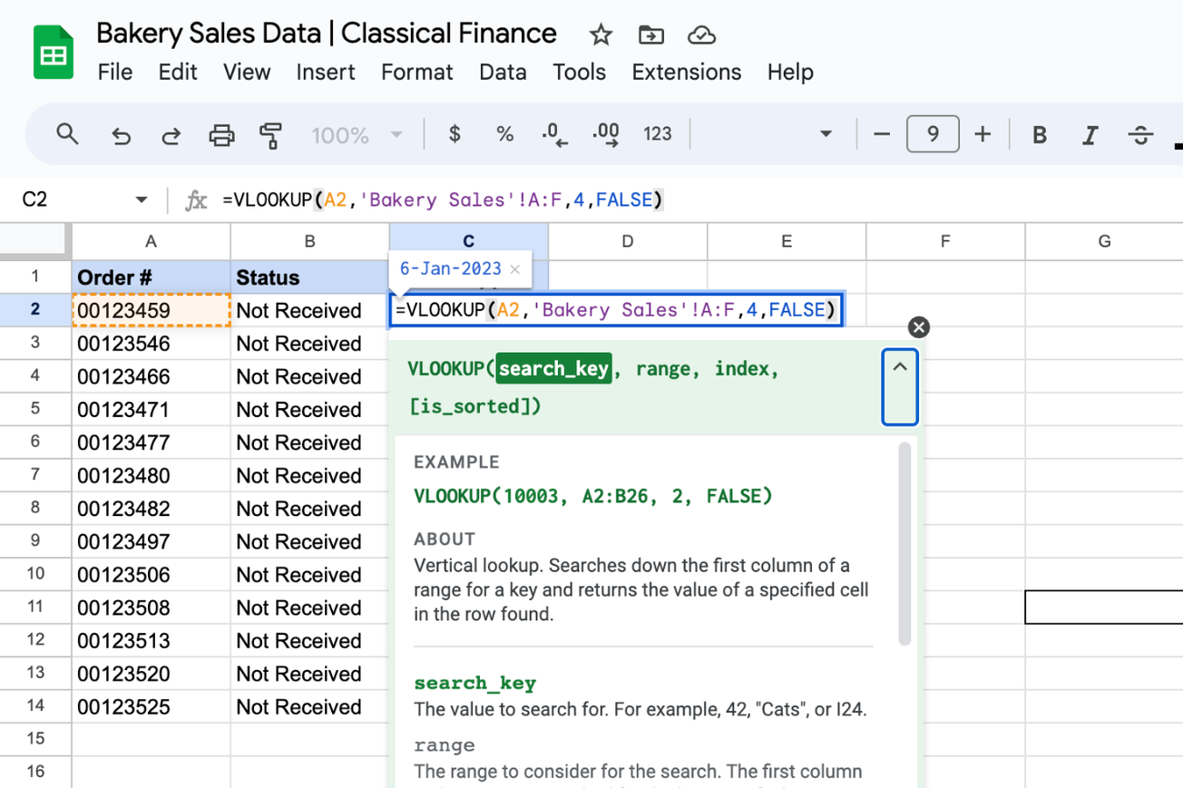
To do this, first we’ll add =VLOOKUP into cell C3, and open brackets to activate the function.
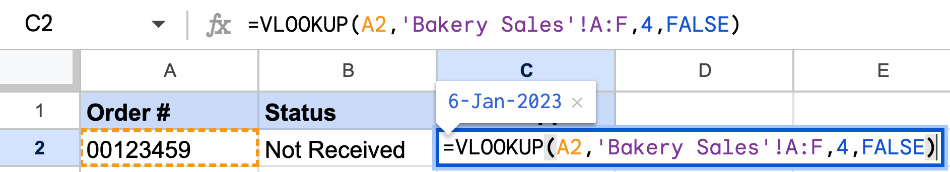
The Search_key in this instance is the order number - that’s the value that we need to look up - we need information that is attributed to this order number. That information is in cell A2 on this sheet, so we can either type in ‘A2’, or just hold down Control and click on the cell we want to use.
Next, we need the range of cells that hold the information that we need. For that, we can head over to the ‘Bakery Sales’ sheet and select each column, while holding Control. We only really need up to the Date Shipped Column, but it doesn’t hurt to select them all. As long as the Order Number column is the first one, that’s all that matters.
Next, we need to ender the index, the column that we need the information from - in this case the Date Shipped column. That is the fourth column along, so we just need to type the number 4 here.
Finally, the data isn’t sorted, so we’ll add FALSE at the end of our formula. Now our formula reads: =vlookup(A2,'Bakery Sales'!A:F,4,false)
Then we hit enter - all of a sudden, the date the order was shipped will appear in the correct cell. To fill this formula down the column, we just need to drag the square in the bottom right of the cell, and it will automatically fill it where we need it. We now have all the data we need for an argument with the courier company!
Example 2
For our second example, let’s imagine our bakery company wants to add a bit more detail to their spreadsheet. They have the quantity of each order, but not the value. Rather than going down and working each one out, for each individual product, they can do a VLOOKUP to automatically work out the value of each order, based on the price of the product that has been ordered.
To illustrate how to do this, we have created a new sheet ‘With Product Prices’, but they wouldn’t need to do this, they could just add it on to the existing sheet.
As you can see, we have added a small table with the prices of each product next to our main data - this is going to be our range that we are going to use to add information into our spreadsheet.
We first have two additional columns - first a column that will display the Unit Price, and then one with the order value. Now we need to populate the Unit Price column with a VLOOKUP formula.

So we’ll start with =VLOOKUP and open our brackets. Then we need to select our Search_key, which for this one will be our Product - that's the key bit of information for which we need to get the price, so we’ll hold Ctrl and select cell B2.
Next, we need the range, so we’ll hold Control again and select all the data in our little table at the side (cells J3:K9). Then we’ll enter the number 2, as we want the information in the second column of our range - the Unit Price. Finally, we just need to finish with FALSE and hit enter - our Unit Price will appear. Make sure to use absolute values for the range so it doesn't change as the formula is copied.
From here, we’re on easy street. We just fill down so the formula goes down to the bottom of our data, and to fill the Order Value column, we need a simple formula - =F2*E2 (or Quantity Purchased multiplied by Unit Price) to give us the over value. Fill that one to the bottom, and we have got the value of every order in a matter of seconds. It’s as easy as that.
Some things to consider when using VLOOKUP
As you can see, using the VLOOKUP formula is in no way as complicated as it might first look. Once you break it down into each section, it really is quite straightforward. There are few things that you should consider though:
Firstly, if the formula goes wrong and shows up the ‘#VALUE!’ error, first check to make sure that you have [is_sorted] as FALSE. Another common mistake is forgetting to enter the Index number - which column within your range that you want to extract the data from.
Another thing to note is that on Google Sheets, the VLOOKUP formula is case insensitive - so it doesn’t distinguish between upper and lower case characters. Something to bear in mind particularly if you use both upper case and lower case for order numbers, for example.
When you hold control and click on the cells that you want to use in the formula, the commas (which act as delimiters) will automatically be added by Google Sheets - but if you find you have an error, go back and check that the commas are separating each element of the formula.
Finally, if you get a #N/A error, double-check your search range as this may be where you have an error - maybe you have added a column since you created the formula which has sent it all out of sync?
Conclusion
We hope that we have given you everything you need to start adding VLOOKUP formulas to your data in order to save yourself a lot of time and hassle. There are so many possibilities when you know how to use VLOOKUP, we are sure you will find plenty of opportunities to use this new skill!
Please leave any comments below, especially if you have any areas of Google Sheets that you would like us to cover in the future.