Are you ready to take your Excel skills to the next level? If so, then you need to learn about conditional formatting. This powerful tool allows you to highlight information in your spreadsheets based on cell rules that you set up. For example, you can use conditional formatting to identify duplicate values, or highlight cells that are above/below a certain threshold. In this guide, we will show you how to use conditional formatting in Excel. We will also provide some examples of how it can be used effectively in business settings.
What Is Conditional Formatting?
Conditional formatting is a feature in Excel that allows you to apply formatting to cells based on certain conditions. For example, you can actually use conditional formatting to highlight all the cells in a column that contain a cell value greater than 1000.
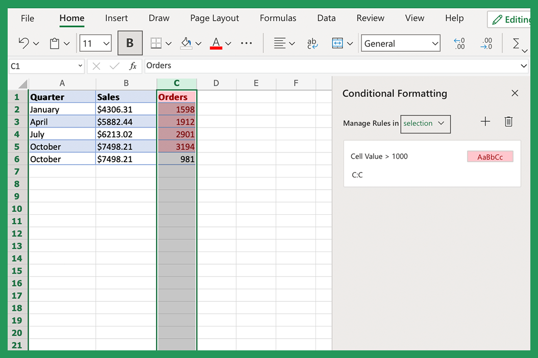
To do this, you would first need to set up a conditional formatting rule. This rule would specify that any cells in the column with a value greater than 1000 should be highlighted. Once the rule is set up, Excel will automatically apply the formatting to all the cells that meet the conditions.
Things To Keep In Mind
There are a few things to keep in mind when using conditional formatting in Excel:
- Conditional formatting rules are applied to a selected range of cells, not just individual cells.
- You can apply multiple rules to the same cell range.
- Cells rules are applied in the order that they are created. If two cell rules conflict, the rule that is higher on the list will take precedence.
- You can use formulas in conditional formatting rules. This allows you to create rules that are based on multiple conditions.
Types of Conditional Formatting Excel Users Love
There are several different types of conditional formatting rules that you can use in Excel. The most common ones are listed below:
- Using the conditional formatting method to highlight cells that meet a certain condition: This type of rule will highlight cells that meet a criteria that you specify. For example, you could use this to highlight all the cells in a column that contain a cell value greater than 1000.
- Using the conditional formatting method to highlight cells that are duplicate values: This type of rule will highlight cells that contain values that are duplicates of other values in the spreadsheet.
- Using the conditional formatting method to highlight cells that are above/below a certain value: This type of rule will highlight cells that are above or below a certain threshold. For example, you could use this to highlight all the cells in a column that are below the average value.
- Using the conditional formatting method to highlight cells that are based on a formula: This type of rule will highlight cells that meet a criteria that is specified in a formula. This is the most versatile type of conditional formatting rule, as it allows you to create complex rules that are based on multiple conditions.
- Using the conditional formatting method to highlight blank cells. These formatting rules will highlight blank cells.
Using Conditional Formatting in Excel to Identify Duplicate Values
One common use for conditional formatting in Excel is to identify duplicate values in Excel spreadsheets. Conditional formatting can be helpful if you are trying to clean up data, or if you need to make sure that there are no duplicate entries in a list.
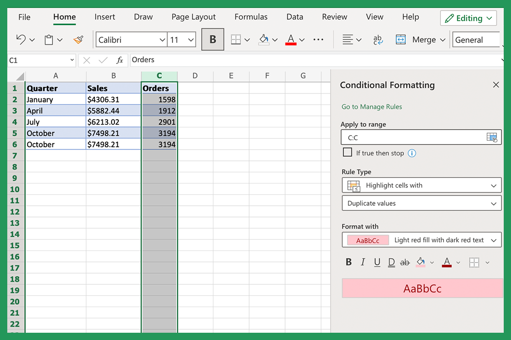
To do this, simply select the cells that you want to check for duplicate values, and then all you do is go to the Home tab > click Conditional Formatting > click Highlight Cells Rules > Duplicate Values.
Finding Unique Values
You can even use conditional formatting to find unique values in a list. To do this, you're going to want to select the cells to check, and then navigate to the Home tab > click Conditional Formatting > click Highlight Cells Rules > Unique Values.
Using Conditional Formatting in Excel to Highlight Cells
Another common use for conditional formatting in Excel, is to highlight cells that are above or below a certain threshold. This can be very incredibly helpful if you are trying to analyze data, and you want to quickly identify outliers.
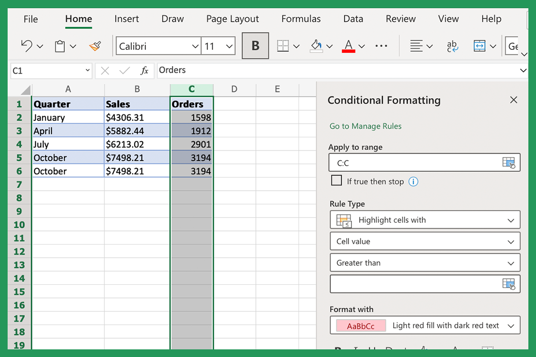
To do this, you first need to select the cells that you want to check, and then click the Home tab > click Conditional Formatting > click Highlight Cells Rules > Greater Than/Less Than.
Highlight Cells Between Values
You can actually use conditional formatting to highlight cells that are between two values. To do this, just select the cells that you want to check, and then click Home > click Conditional Formatting > click Highlight Cells Rules > Between.
Highlighting Top/Bottom 10 (or 10%) Values
Another common use for conditional formatting is to highlight the top or bottom 10 (or 10%) values in a list. This can be beneficial if you are trying to find the highest values or lowest values in a set of data. To do this, you've got select the cells that you want to check, and then go to the Home tab > click Conditional Formatting > Top/Bottom Rules > Top 10 Items.
You can also highlight the bottom 10 items by selecting Bottom 10 Items from the Top/Bottom Rules menu. Want to highlight blank cells? You can do that, too!
Creating Data Bars with Conditional Formatting in Excel
You can also use conditional formatting to create data bars. Data bars can be helpful if you want to quickly visualize the data in your spreadsheet.
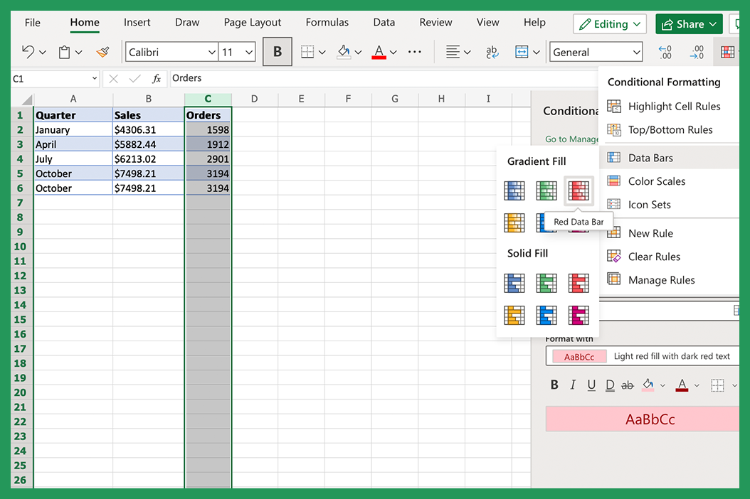
Select the cells that you want to check, and then go to the Home tab > click Conditional Formatting > Data Bars > Gradient Fill.
Creating a Color Scale Using Conditional Formatting in Excel
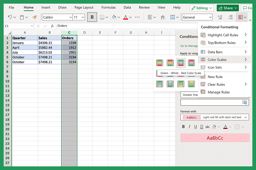
Another way to visualize data is to use a color scale. Color scales are a type of conditional formatting that allows you to visually compare data points. For example, you can use a color scale to quickly see which cells are higher or lower than other cells.
Color scales will color the cells in your spreadsheet based on their values. To create color scales, select the cells that you want to check, and then click on the Home tab > click Conditional Formatting > Color Scales.
Creating Conditional Formatting Icon Sets in Excel
You can also use conditional formatting to create icon sets. This will insert icons into the cells in your spreadsheet based on their values.
To create conditional formatting icon sets, select the cells that you want to check, and then navigate to the Home tab > click Conditional Formatting > Icon Sets.
Using Conditional Formatting to Visualize Data
In addition to the uses mentioned above, conditional formatting can also be used to visualize data in various other ways. This can be helpful if you want to create a dashboard or report that is easy to understand at a glance. In order to do it, select the values or cells that you want to format, and then head on over to the Home tab > click Conditional Formatting > Data Bars > Gradient/Light Red Fill.
Creating Heat Maps with Conditional Formatting in Excel
You can also use conditional formatting to create a heat map. This is a type of visualization that uses different colors to represent different values.
To create a heat map, select the certain cells that you want to format, and then to create the color scales go to the Home tab > click Conditional Formatting > Color Scales > 3-Color Scale.
Should You Apply Conditional Formatting in Excel?
As you can see, there are several ways to use conditional formatting in Excel. Whether or not you should use it will depend on your specific needs.
If you need to quickly analyze selected data or find specific values, then conditional formatting can be a helpful tool. However, if you want to create a dashboard or report, you might want to consider using another visualization tool.
Is Conditional Formatting for Excel Users Only?
No, conditional formatting is not just for Excel users. You can apply conditional formatting in any program that supports the use of cells and cell values. This includes programs like Google Sheets, Numbers, and Quattro Pro.
How To Reverse Conditional Formatting Mistakes?
If you make a mistake when you apply conditional formatting in Excel, don't worry! You can always undo your changes by going to the Home tab > click Conditional Formatting > Clear Rules > Clear All Rules from Sheet. This will remove all conditional formatting cells rules from the sheet, so you can start again from scratch.
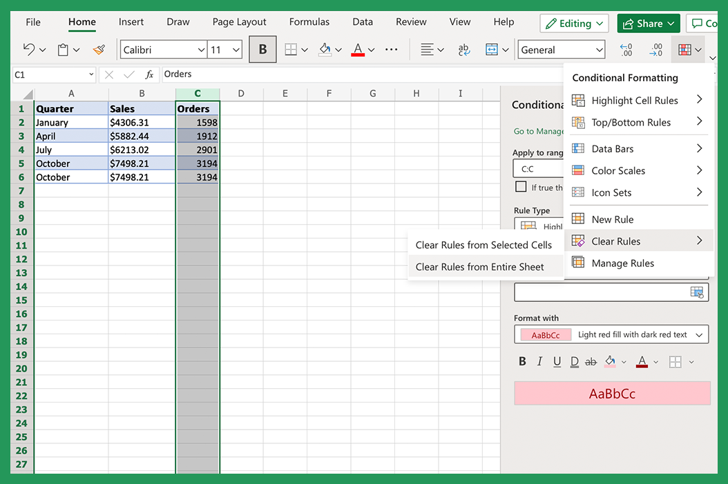
You can also remove conditional formatting from a cell/range of cells by selecting the cells that you want to edit or remove the conditional formatting from, and then going to the Home tab > click Conditional Formatting > Clear Rules > Clear Rules from Selected Cells.
What Is A Conditional Formatting Rule Dialog Box?
A conditional formatting rule dialog box is a tool that you can use to create and edit conditional formatting rules. To open the conditional formatting rule dialog box, select all the cells that you want to format, and then go to the Home tab > click Conditional Formatting > New Rule.
The conditional formatting rule dialog box will allow you to specify the type of conditional formatting that you want to apply, as well as the conditions that will trigger the formatting. For example, you can use the conditional formatting rule dialog box to create a rule that will highlight cells that contain numbers greater than 100.
You can also use the conditional formatting rule dialog box (or dialogue box) to edit existing conditional formatting rules. To edit, select all the cells that you want to format, and then go to the Home tab > Conditional Formatting > click Manage Rules or Edit Rule. This will then open the Conditional Formatting Rules Manager, which will allow you to edit, delete, manage rules or disable existing conditional formatting rules.
When Should You Use Conditional Formatting in Excel?
Conditional formatting is a great way to highlight important data points, make your data easy to understand, and find errors in your data. However, it's important that you are applying conditional formatting in Excel sparingly, as too much can make your data hard to read.
If you're not sure whether or not you should use conditional formatting in Excel, ask yourself these questions:
- Will conditional formatting help me highlight important data points?
- Will conditional formatting make my data easy to understand at a glance?
- Will conditional formatting help me find errors in my data?
- Will conditional formatting help me spot trends in my data?
If you can answer yes to any of these questions, then conditional formatting may be the formatting option to consider.
When Not To Use Conditional Formatting?
Conditional formatting is a powerful tool, but it's not always the best solution. In some cases, it may be better to use a different data visualization technique, such as using colors, shapes, or icon sets.
How To Remove Conditional Formatting in Excel
If you want to go about removing conditional formatting in Excel from a corresponding cell/ range of selected cells, simply select the cells that you want to remove the formatting from, and then go to the Home tab > click Conditional Formatting > Clear Rules > Clear Rules from Selected Cells.
You can also clear all conditional formatting from a sheet by going to the Home tab > click Conditional Formatting > Clear Rules > Clear All Rules from Sheet.
Tips To Make The Most Out Of Conditional Formatting
Here are a few tips to help you make the most out of conditional formatting in Excel:
- Use conditional formatting sparingly. If you use too much, it can be hard to read your data.
- Use conditional formatting to highlight important data points.
- Use conditional formatting to make your data easy to understand at a glance.
- Use conditional formatting to create heat maps and data visualization.
- Use conditional formatting to find errors in your data.
- Use conditional formatting to spot trends in your data.
- Use conditional formatting for data validation.
Conditional formatting is a powerful and valuable Excel tool that can be used to improve the clarity and usefulness of your data. When used sparingly, conditional formatting can help you highlight important data points and make your data easy to understand at a glance.
When used correctly, it can also be used to create heat maps and data visualizations. And when used to find errors in your data, it can help you spot trends and improve the accuracy of your data (data validation).
So, if you're not using conditional formatting in Excel already, now is the time to start applying some cell rules!
Conclusion
As you can see, there are so many various, diverse ways that you can apply conditional formatting based on your own cell rules. Cell rules are the conditions that you specify for conditional formatting.
By understanding how to use conditional formatting rules, you can take your spreadsheet skills to the next level. So what are you waiting for? Start experimenting with conditional formatting today!