The VLOOKUP function in Excel can be used to look up specific information in a data set. The function searches for a value in the first column of a data set and returns the corresponding value from another column in the same row. The VLOOKUP function can be used to look up values in a table, a named range, or an array.
The VLOOKUP function stands for ‘Vertical Lookup,’ and is typed out like this: =VLOOKUP.
And here is the syntax of the VLOOKUP formula and its components:
=VLOOKUP(lookup_value, table_array, col_index_num, [range_lookup])
We’ll break each part of this function below so you know what information the VLOOKUP formula is seeking, and what info you’ll be inputting into each part.
What Is the VLOOKUP Used For?
The primary purpose of the VLOOKUP function is to help you retrieve information, especially if you’re always searching for the same type of data in a really large spreadsheet. So the VLOOKUP function can help you find data much quicker than scrolling through. For example, you can use the phone number of a client using their last name, or the price of an object in your inventory using its item code.
When you use the VLOOKUP formula in Excel, it will search for a certain value in a vertical column (or table array) of a table or range in your spreadsheet. It will then return a value from a different column number in the same row. You are providing it with a value, where you want to look for it, and the column range that contains the value to return.
Another way to say it is this function acts somewhat like a phonebook, where you are using a column in the table with the information you know (the person’s name) to find the information you don’t know (their phone number).
Getting Started: Defining Each Part of the VLOOKUP Formula
Let’s define what each section of the VLOOKUP formula actually means. Again, here is what the full syntax looks like:
=VLOOKUP(lookup_value, table_array, col_index_num, [range_lookup])

- Lookup_value: This is the lookup value, or the value you are searching for. It’s the value Excel will find a match for in the left most column of your table range. It is directly followed by a comma.
- Table_array: This provides Excel with where you want to search. It’s the columns in the lookup table range. The lookup table range is directly followed by a comma.
- Col_index_num: This part is the column that contains the result. Excel will search this column to find the match to your lookup value. It is directly followed by a comma.
- [range_lookup]: This optional part indicates to Excel whether you want an exact match to the lookup value, or an approximate match. TRUE indicates an approximate match, and FALSE indicates an exact match. Note: If you choose not to enter anything here, it will default to TRUE.
Note: VLOOKUP will only work properly if your data is neatly arranged as a vertical table with rows. The value you are looking for must be in the left most column of the cell range, to the left of the return value you’re looking for.
How to Use the VLOOKUP Function
Ready to enter all of the lookup values into the VLOOKUP function? Let’s get started.
Step 1: VLOOKUP
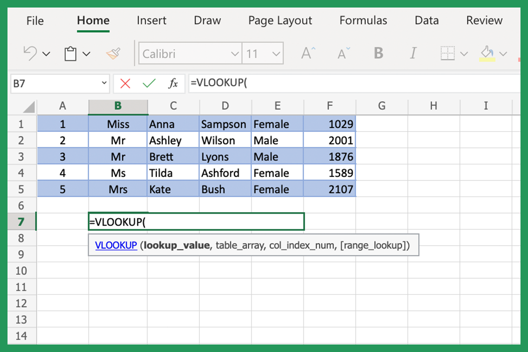
In the Formula Bar at the top of the spreadsheet, type in =VLOOKUP(). The other parts will go in between the parentheses.
Step 2: Lookup Value
Starting inside the parentheses, enter your lookup value. A quick way to do this is by double clicking on the VLOOKUP command and selecting the cell the search value will be entered. You can also manually input the actual lookup value or just the empty cell that will hold a value.
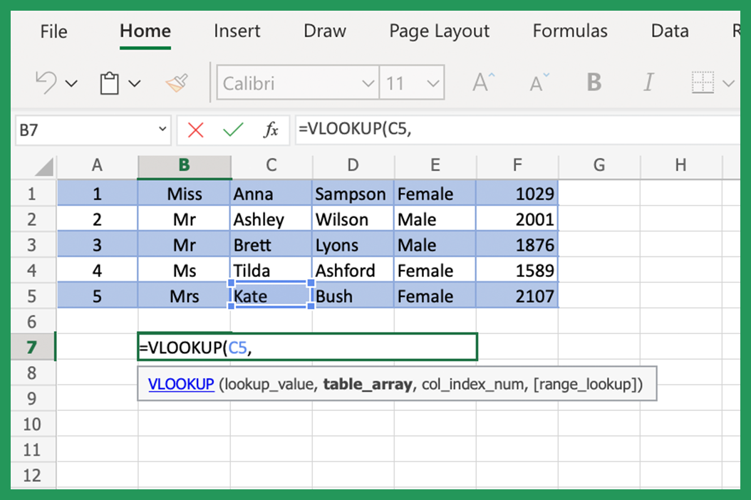
Place a comma directly after the lookup value. Here is an example of what it might look like: =VLOOKUP(F10,
Step 3: Table Array
Next, input the table array, or the range where Excel needs to search for the match to your lookup value. Separate each exact value with a colon, and end the array with a comma. It will look something like this: =VLOOKUP(F10,C2:E30,
Step 4: Column Index Number
Next, you will enter the column index number. Here is where you will input the numeric value of the column you think the information you need will be found, such as column number ‘2’ or ‘4’.
This column must lie to the right of your lookup values. Make sure you place a comma directly after it. It will be typed like this: =VLOOKUP(F10,C2:E30,4,
Step 5: Range Lookup
Finally, you will input the range lookup value, which will either be the word TRUE or FALSE. TRUE will find approximate matches for your lookup value, and enter FALSE to search for exact matches.
This step is optional, but keep in mind if you leave it blank, the VLOOKUP Excel formula will process with a TRUE as default. It will look something like this: =VLOOKUP(F10,C2:E30,4,FALSE)
Troubleshooting Tips
Here are a couple issues you may run into with the Excel VLOOKUP function.
- Is the function just not producing any results, or coming back with an error message? Make sure you check your computer’s Language Settings. Some settings will have you place a comma [ , ] after each argument, and some will need a semicolon [ ; ]. It’s more standard to see commas, though.
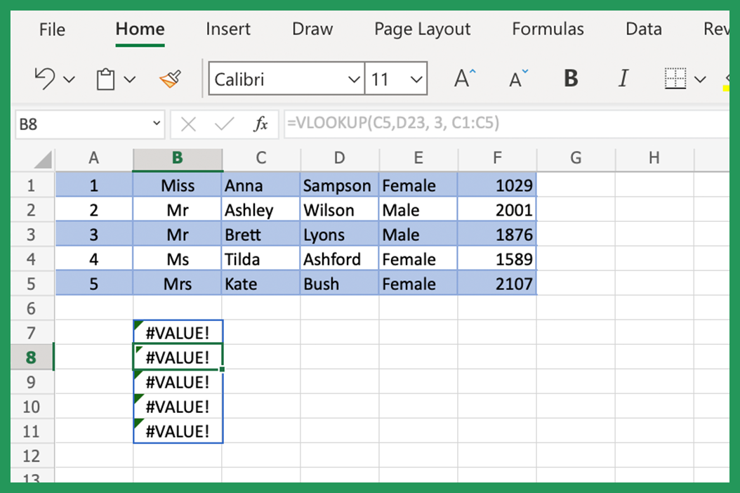
- Do you keep ending up with an #N/A error? This may be happening because of the FALSE that you may have inputted into the formula. If an exact match for the value you’re looking for doesn’t exist, or you’ve set your range incorrectly and it simply can’t find the correct answer, it will produce this #N/A error.
Note:
- Do you need to perform a Horizontal Lookup, rather than a Vertical Lookup? You can use the HLOOKUP functionin Excel. This will look through the horizontal rows in your table.
- Want to learn a convenient hack? If you want to take your value search further than just strictly VLOOKUP or HLOOKUP, there’s a newer Microsoft Excel function that allows you to do this: XLOOKUP. This function will have Excel look through any direction of columns and rows, and return exact matches by default instead of approximate matches. Only stipulation is you’ll need a Microsoft 365 subscription, and the latest version of Office.
Does VLOOKUP Support Approximate Match?
By default, VLOOKUP uses an approximate match in Excel. What does this mean? It means that if the value you're looking for isn't an exact match, it will still return a value - AKA approximate match.
For example, if you're trying to look up the number 5 and all your values are in increments of 10 like 10, 20, 30, 40, VLOOKUP will return the value 10.
You can change this by adding a fourth argument to your function. The 4th argument is either TRUE or FALSE. If you set it to FALSE, VLOOKUP will only return an exact match, not an approximate match.
Using VLOOKUP to Find Exact Match
If you want to find an exact match using VLOOKUP, you need to set the 4th argument to FALSE.
You can also use MATCH to find an exact match and then use that result with INDEX to get the value you want.
How Do I Use VLOOKUP With Multiple Criteria?
If you want to use VLOOKUP with multiple criteria, there are a couple ways you can do this.
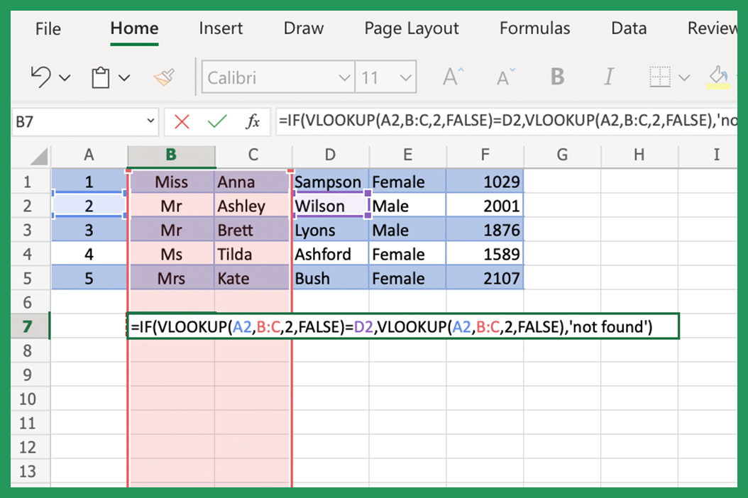
The first way is by using the IF formula. This function will check if your first criterion is met, and then return the corresponding value. You can then use another IF formula to check for your second argument. For example:
=IF(VLOOKUP(A2,B:C,2,FALSE)=D2,VLOOKUP(A2,B:C,2,FALSE),'not found')
The second way is by using the INDEX and MATCH function. This function will first check if both criteria are met and then return value.
=INDEX(B:C,MATCH(1,(A2=B:B)*(D2=C:C),0))
Both of these methods will require that your data is sorted. Sorting your data will make it easier for Excel to find the values you're looking for.
How Do I Use VLOOKUP to Find the Closest Match?
If you want to find the closest match, you can use the VLOOKUP function with the MATCH function.
The MATCH function will return the position of a value in an array or range. You can then use this position to return the corresponding value from your array or range.
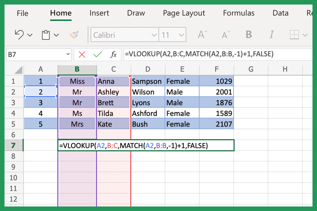
=VLOOKUP(A2,B:C,MATCH(A2,B:B,-1)+1,FALSE)
The Excel MATCH function has a third argument that allows you to specify whether you want an exact match or an approximate match.
If you want an exact match, you would use a 0 as the third argument. If you want an approximate match, you would use a 1 as the 3rd argument.
However, if you want to find the closest value, you would use a -1 as the third argument.
This will tell Excel to find the largest value that is less than or equal to the value.
How Do I Use VLOOKUP to Return Multiple Values?
If you want to return multiple values, you can use the VLOOKUP function with the INDEX and MATCH function.
INDEX will return a value from a given array or range. You can use this to return multiple values from your array or range.
=VLOOKUP(A2,B:C,MATCH(A2,B:B,-1)+1,FALSE)
Using VLOOKUP for Partial Matches
If you want to use VLOOKUP for partial matches, you can use the wildcard character (*). The wildcard character can be used to replace any characters in your lookup data.
You can also use the question mark (?) wildcard character to replace a single character.
Find Duplicate Values
If you want to find duplicate values, you can use the COUNTIF function.
COUNTIF will return the number of cells that contain a given value. You can use this to check if a value exists more than once in your table.
VLOOKUP Function Fails to Be Aware Of
Column Insertions
If you insert a column next to the lookup column, the VLOOKUP function will continue to look in the original column for the value.
To fix this, you can use the INDIRECT function. The INDIRECT function returns a cell reference or range of cells.
You can use this function to dynamically reference cells. This means that if you insert a column number, the reference will change automatically.
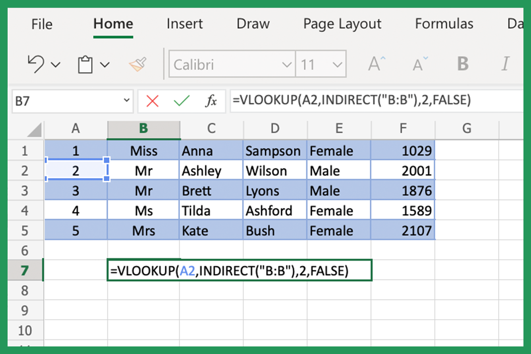
=VLOOKUP(A2,INDIRECT("B:B"),2,FALSE)
The INDIRECT function takes a string as an argument. The string is the reference to the cell or range of cells.
You can use the Excel INDIRECT function with the VLOOKUP function to dynamically reference a cell or range of cells. This means that if you insert a column in the table, the reference will automatically update. Make sure you don't include the FALSE part of the syntax, with the INDIRECT reference in double quotes.
VLOOKUP Only Returns First Match
VLOOKUP only returns the first match it finds. If there are multiple matches, it will only return the first one.
To fix this, you can use the INDEX and MATCH formulas. INDEX returns a value from a given array or range. You can use this to return multiple values from your array or range.
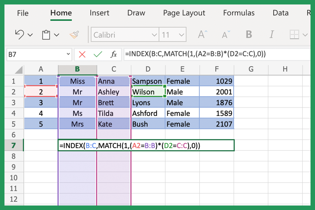
=INDEX(B:C,MATCH(1,(A2=B:B)*(D2=C:C),0))
The Excel MATCH formula returns the position of a value in an array or range. You can then use this position to return value from your array or named range.
Conclusion
There you have it! We hope this guide has covered everything you need to know about the VLOOKUP function in Microsoft Excel. VLOOKUP works perfectly in Excel, so long as you're up to speed. As always, if you have any questions, feel free to reach out via our Contact Us page. We’re happy to help!