The Xlookup excel function is a powerful and flexible search tool. It allows you to find values from a specific range of cells and has combined the features of the Vlookup and Hlookup functions, making it a more versatile tool for data lookup.
Xlookup provides more value than its predecessors. The new and improved function allows the user to quickly find a value within a dataset – vertical lookup or horizontal lookup – and return the corresponding value in another specified column or row. Should there be more than one result, the last result is used.
Introduced within Microsoft 365 back in 2020, Xlookup is considered a relatively new excel function. For now, it's only available on Office 365; however, if you still cannot locate it, there's a nifty little trick that just might work for you. First, click on the File tab and then navigate toward Account. From there, you might notice an option on the bottom labeled Office Insider – this will help you locate the Xlookup function.
The XLOOKUP Function Syntax in Excel
To start, let's take a closer look at the specific syntax before we dive in further:
=XLOOKUP (lookup, lookup_array, return_array, [not_found], [match_mode], [search_mode])
As you can see, there are a few required arguments for the function:
- Lookup: The value that we want to find in our lookup array
- Lookup Array: The range of cells where we want to search for our lookup value
- Return Array: The range of cells that contains the corresponding values that we want to return
The following are optional arguments:
- Not_found – will only populate if no match is found. Past lookup functions returned an #N/A error. However, Xlookup supports other values. For example, Xlookup can return a Boolean value such as True or False, a cell reference, or a text value such as Not Found, No Match, or No Result.
- Match_code – 0 is the exact match; -1 is the exact match function or the next smallest; 1 is the exact match or the next larger value; 2 is a wildcard match function. It can be used as a fifth argument.
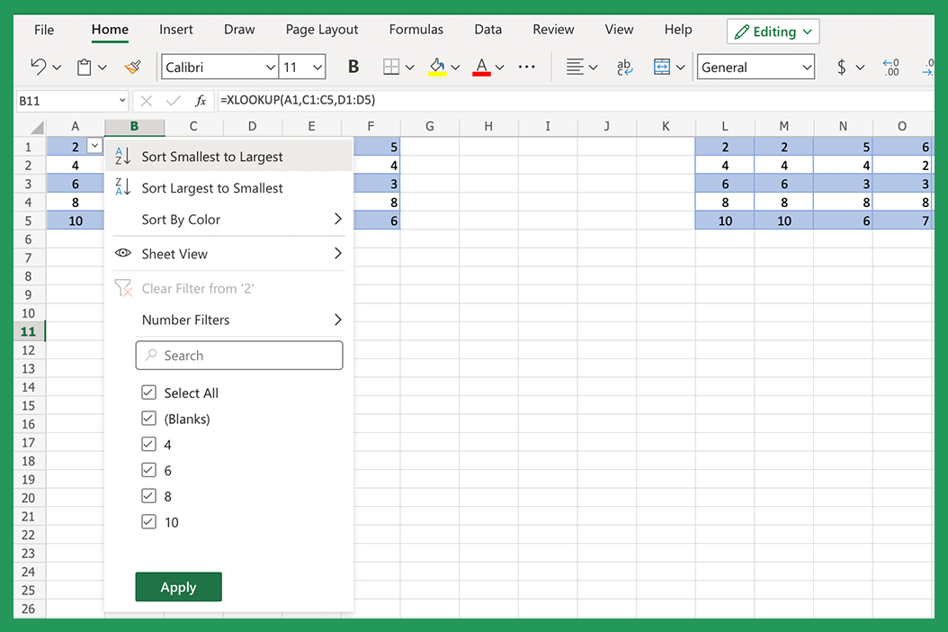
- Search_mode – by default, search mode using Xlookup returns the first value. To change this, use the following options: 1 search from first; -1 means to search from last; 2 is a binary search in ascending order; -2 is a binary search in descending order. It can be used as a sixth argument.
What is Binary Search Mode?
Binary search mode is a faster method to search for exact matches within a sorted dataset. When using this method, you must first sort the table array in ascending or descending order.
What is Reverse Search Mode?
Reverse search mode begins the search at the end of the array and moves backward. Use this option when your lookup value is close to the end of the array, as it will be faster than the default search mode.
A Step-By-Step Guide to Using the Xlookup Function in Excel
The following steps will guide you through the Xlookup function.
Select Cell
Start by opening the excel spreadsheet with your data set, then select an empty cell. To add the new formula to the empty cell, click on the formula bar in the ribbon bar to start editing. The cell is active and ready for editing when the blinking cursor is visible on the ribbon.
Narrow Down the Search Criteria
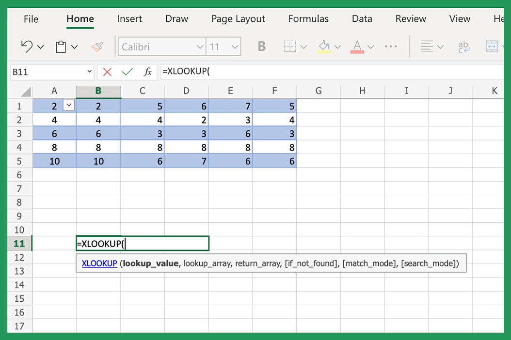
As explained above, Xlookup has a specific structure that must be followed for the formula to provide the expected results over invalid results. Commas separate each individual argument within the formula. To start, type in =XLOOKUP( into the ribbon bar.
The next step asks for the lookup criteria or the data you're searching for using the formula. The Xlookup function supports numbers and text strings, but most users prefer to specify a cell reference. One benefit is that it allows the user to change the lookup criteria without adjusting the entire formula.
We'll continue with selecting a cell rather than specifying numbers or a string of text. For example, if the lookup criteria are located in cell A1, the formula will begin to look as follows: =Xlookup(A1,. This is because the Xlookup excel function will attempt to find an exact match in the data set we'll designate next. Use the appropriate match_code argument to find approximate matches instead of exact matches for all other match types.
Determine the Data Set
With the lookup value identified, you'll need to specify the lookup_array and return_array cell ranges, or in other words the set of data you'll be searching through.
The lookup_array will be the row or the column which will contain the search query specified in the lookup criteria. For those using the match_code option, this will also include approximate match results. The return_array is the row or column you want to see as the search result.
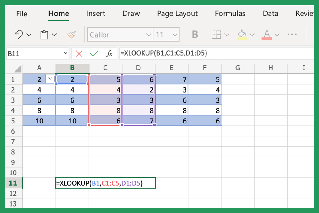
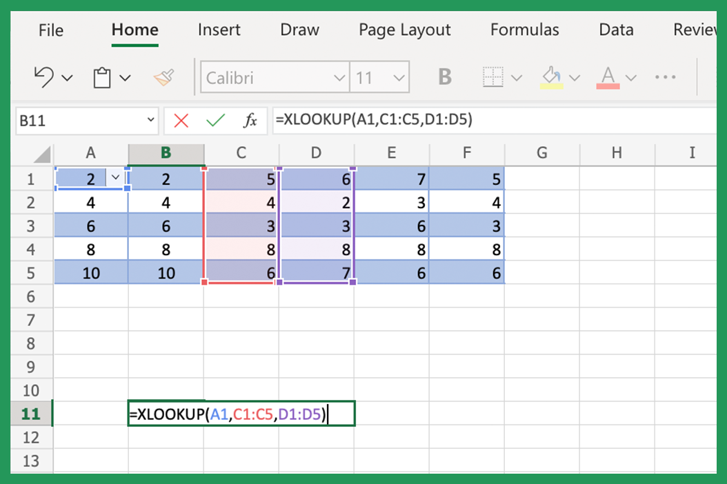
An example of the syntax so far would look like this: =Xlookup(B1,C1:C5,D1:D5). This means that the Xlookup function will look to find an exact match of cell B1 within cells C1 through C5 and then return the information in D1 through D5 if a match is found.
This is the simplest Excel formula form, which does not produce custom error messages, does not use a different search value type, and does not change the search order. Continue to add to your formula if other options are desired.
Adding a Custom Error Message in Excel
For those instances where Xlookup tries to find an exact match but cannot find it in the lookup_array, excel returns an #N/A error message. To ensure that doesn't happen, you'll need to add a not_found argument into the original Xlookup formula.
As mentioned earlier, there are a couple of options when it comes to setting the not_found argument; the next optional parameters in the Xlookup formula are:
- A numerical value (such as 1)
- A string in quotes (such as "not found")
- A Boolean value (True or False)
- Cell reference (which contains the information to display)
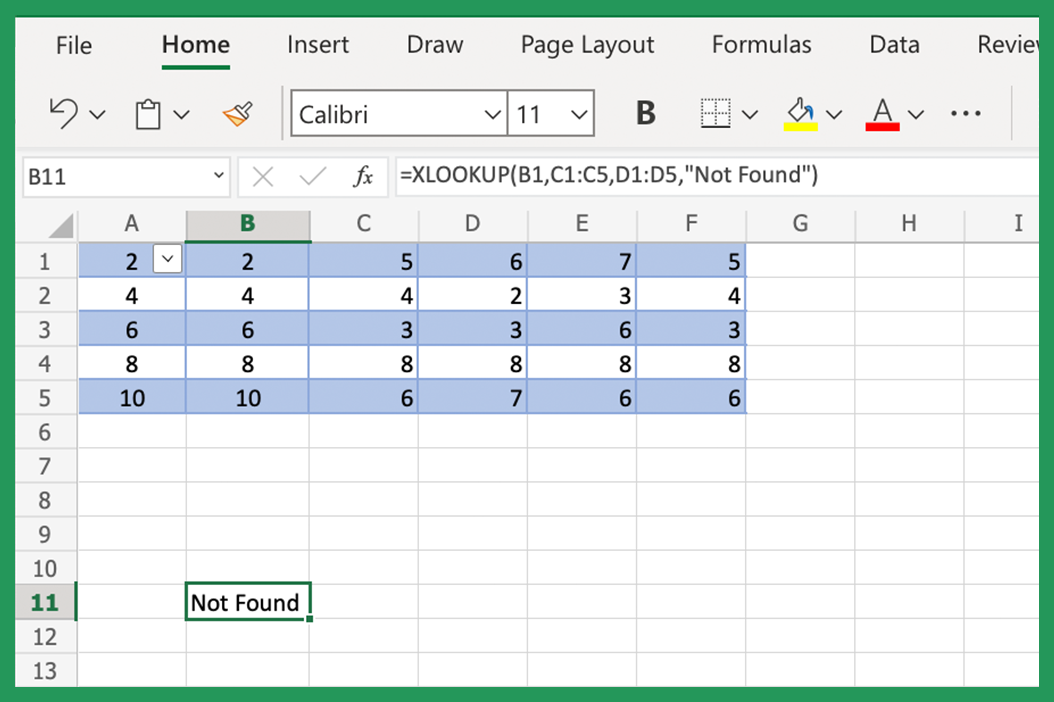
Changing the formula to the following =XLOOKUP(B1,C1:C5,D1:D5,"Not Found") would allow the original #N/A error to show as not found if Excel cannot find the exact match to the lookup value in A1.
Exact Match Type, Approximate Match Type, or Wildcard Match Searches
Though the Xlookup excel formula is designed to find an exact match, the match_mode argument will change the Xlookup defaults.
The match_mode comes with four possible values:
- 0 for an exact match; this is also the default and doesn't need specification
- -1 for an exact match or the next value below
- 1 for an exact match or the next value above
- 2 for partial matches which use asterisks, tildes, or question marks as a wildcard match
Using the above formula as a continuing example, if the formula is now adjusted to show =XLOOKUP(B1,C1:C5,D1:D5,"Not Found",2), the search will now support a wildcard query. If the value in the lookup cell (B1) now reflects a wildcard or is specified in the formula in a text value, the Xlookup formula finds the nearest matching value.
In the following example spreadsheet, B1 has the following information: B*. The Excel formula will look to find any partial matches or a lookup value that starts with the letter B in the lookup_array. And will result in displaying the return_array information. To make sure you get the correct lookup value, you need to consider adding in a search_mode to change the search order.
Determine the Value Return Order
The search_mode option is the last argument supported by the Xlookup formula. Simply put, this argument will change the order in which Xlookup grabs the multiple results. As a default, Excel tries to match the first possible value, but this can be changed.
There are four values for the search_mode argument:
- 1 searches for the first possible lookup value
- -1 reverses the order to search for the last possible value
- 2 searches in binary with ascending order
- -2 searches in binary with descending order
The Xlookup function is great for finding specific information in large data sets when an exact match is needed. The different options allow for flexibility in your search. This is dependent on what is being looked for and how important an exact match may be.
One downside to remember is that the Xlookup function isn't supported in versions before Excel 365. So, if you need to use this function and don't have the supported version, you can try one of these alternatives:
-Index/Match
-Vlookup
These lookup functions are similar to Xlookup but may not offer as much flexibility. Another downside is that these formulas can be longer and more complex than Xlookup, which may make them more difficult for some users.
If you need to use the Xlookup function but don't have Excel 365, consider upgrading your software. If that isn't possible or you prefer not to, Index/Match and Vlookup are viable alternatives that may get the job done.
What Lookup Values to Use in Excel?
When using the Xlookup function, it's important to decide what lookup value will be used. This can be a specific lookup value, cell references, matching value, or a text string.
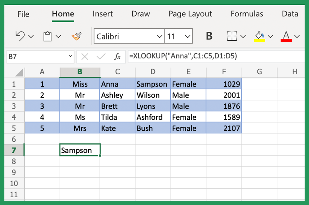
A specific lookup value is a number or text value entered into the formula. For example, if you wanted to look up the last name for the first name "Anna," the formula would be written as =XLOOKUP("Anna",C1:C5,D1:D5).
A cell reference is when the lookup values are pulled from another cell.
A text value is when a wildcard is used as the lookup value. You can do this by adding an asterisk (*) before and after the text string or lookup values. For example, if you wanted to find all of the last names that begin with "Bu," the formula would be written as =Xlookup("Bu*",C1:C5,D1:D5).
It's important to note that the order of the arguments matters when using the Xlookup function. The first argument must be the lookup value, followed by the lookup array, return array, match mode, and search mode.
How To Return Multiple Values Using Xlookup?
One great feature of the Xlookup function is that it can return multiple values. This is done by using an array as the return array argument.
To do this, simply enter the dynamic array into the return array argument. For example, if you wanted to return both the first and last name for "Sampson," the formula would be written as =Xlookup("Sampson",C1:C5,{B1:B5,D1:D5}).
This is a great way to avoid using multiple lookup formulas when you use the Xlookup function, and can help make your Excel spreadsheet more efficient.
It's important to note that the multiple criteria array must be entered in the same order as the lookup array. So, if the first names are in column B and the last names are in column D, the multiple criteria array must be entered as {B1:B10,D1:D10}.
Can You Use Index and Match with Xlookup?
Yes, you can use the Index and Match functions with Xlookup. They can be used together to create a more powerful lookup formula.
To do this, simply nest the Index and Match mode lookup functions inside of the Xlookup function. For example, if you wanted to return a matching value for the last name of "Bush," the nested Xlookup functions would be written as: =XLOOKUP("Bush",D1:D5,INDEX(D1:D5,MATCH("Kate",C1:C5,0))).
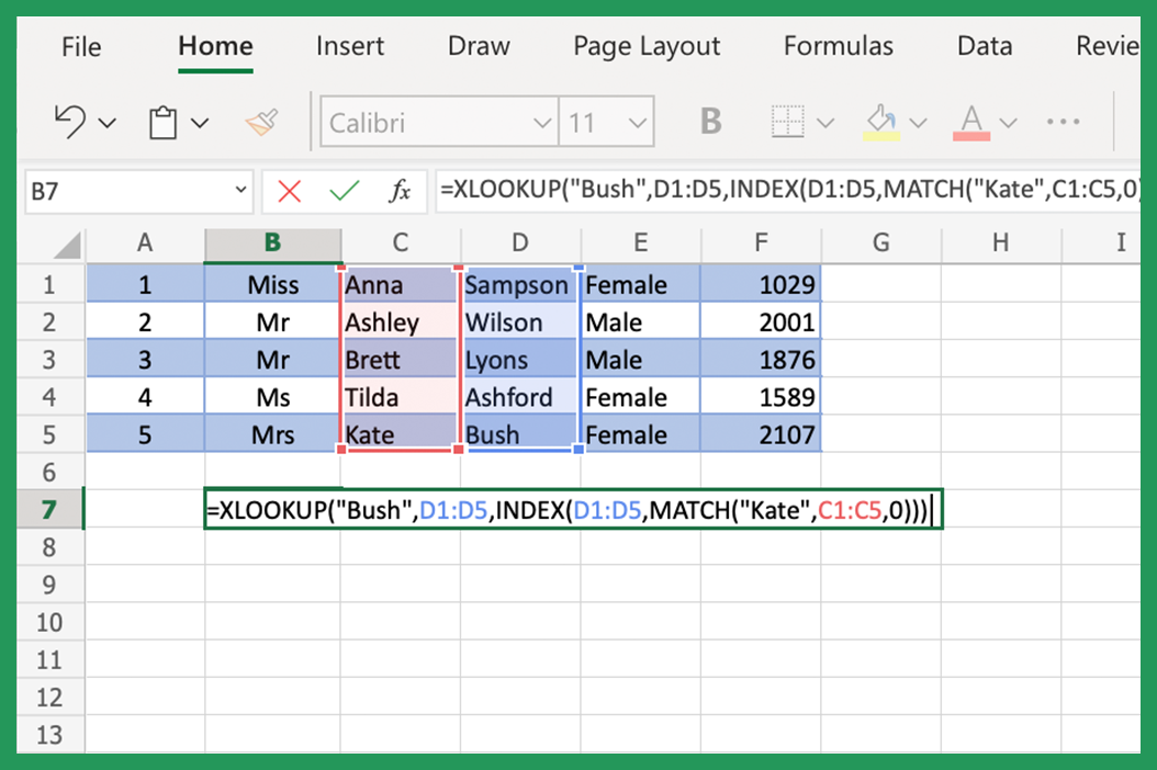
This formula uses the Index function to return the last name from column D and the Match mode function to find the same row number where "Bush" is located in column D.
What Is Horizontal Lookup?
Horizontal lookup is a type of VLOOKUP function in excel which is used to find things in a table by looking horizontally, i.e., left to right, instead of the conventional way, which is top to bottom. Horizontal lookups come in handy where the data is laid out horizontally, i.e., in rows instead of columns.
Final Thoughts
The Xlookup excel function provides a certain amount of flexibility within your Excel spreadsheet. One that is simply not found in its predecessors. Though the Xlookup formula is a huge step forward in data analytics, allowing users to search through large amounts of data quickly, it is not backward compatible. Remember that the data will show errors if a file is created and uses the Xlookup formula, which is then opened without them.
When comparing with other lookup functions in Excel, Xlookup provides the flexibility to look through data in rows or columns. Unlike Vlookup and Hlookup functions, which are restricted to either columns or rows, Vlookup searches through columns, and Hlookup searches through rows.
One last thing to keep in mind when using Xlookup is to keep in mind optional parameters and the expected matching result. The results will be much different than expected if you use the wrong search value, order, or match modes, though there won't be any obvious errors. Have a go at a couple of Xlookup examples to double-check your work if you find yourself working with vast amounts of data.
In other words, the Xlookup is the new and improved search function within newer Microsoft Excel programs. A great addition to data analytics, this single formula provides flexibility unlike any other in Excel. Xlookup works beautifully, so long as you make sure you're getting the syntax right and avoiding invalid results.
In addition, this new function makes working with large quantities of data relatively easy and user-friendly.