Drop down lists in excel are used to create menus from which you can select a value. This feature is helpful if you have many different entries in a column and you want to quickly view or work with a specific subset of those entries.
We'll look at how to use drop downs in a variety of other ways too, including generating a picklist for users to choose from. We will be showing you how to remove drop down lists too.
| # | Example |
|---|---|
| 1 | Filtering Data |
| 2 | Creating A Picklist |
| 3 | Removing A Drop Down |
1. Filtering Data
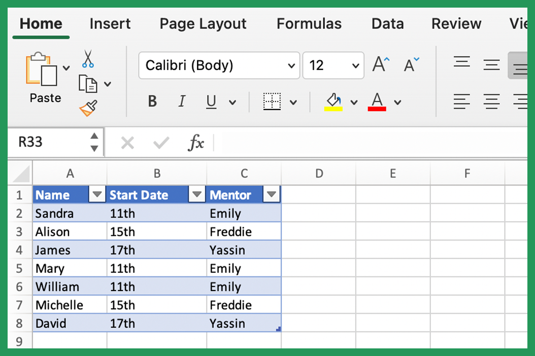
Imagine you're creating a new starters' list for your company. You have three columns: name, start date, and mentor. We'll see if we can filter the data in Microsoft Excel to show just those who will began on the 17th.
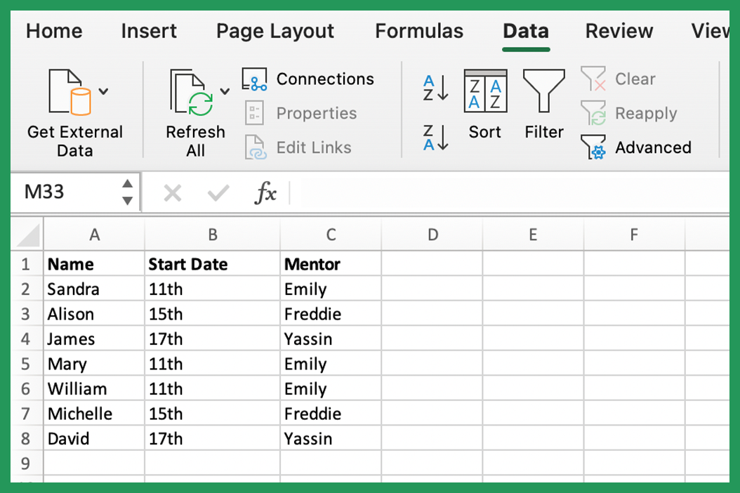
The fastest way is to create a table is to press Ctrl + T or Control + T on mac and a table will be created with drop down lists.
We then have drop down lists on all three columns. Press the arrow on the "Start Date Column".
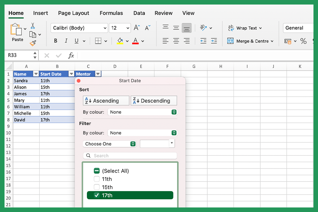
All of the data will be selected automatically. Adjust the checkbox so that only the data for the 17th is showing.
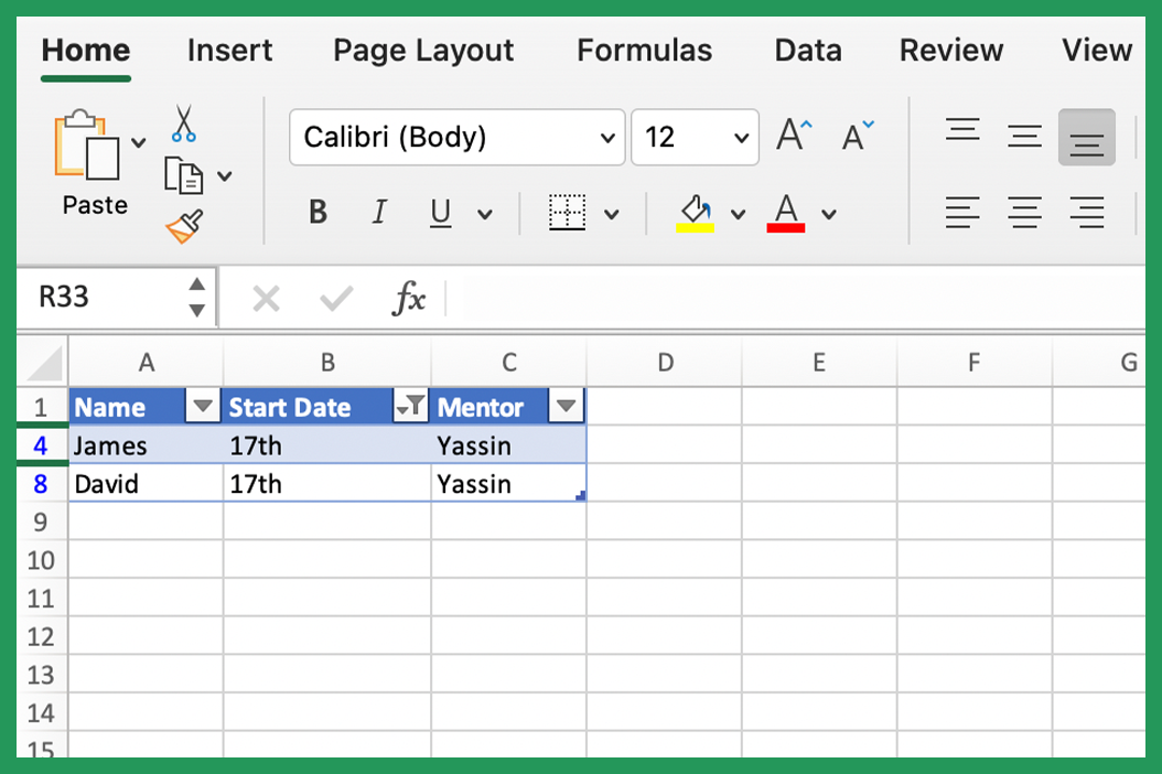
We can now see that James and David are starting on the 17th and their mentor will be Yassin. Result!
2. Creating A Picklist
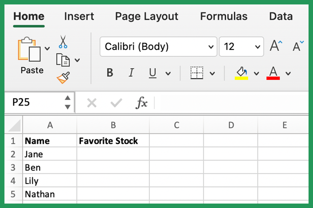
Creating a picklist in Excel is useful for data entry efficiency and avoiding typographical errors. In this example we will create an input sheet where participants select their favorite stock.
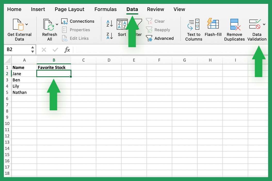
Create a list of names and add a column for 'favorite stock'.
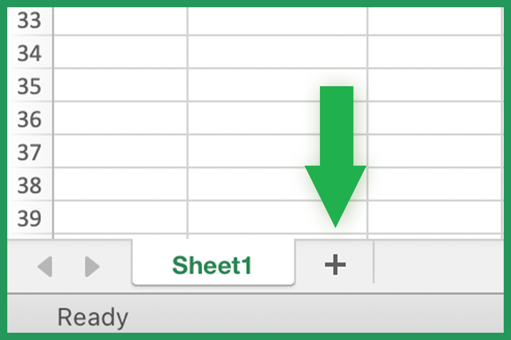
For our picklist we will create a new worksheet in our workbook to keep things tidy. We can do this by pressing the plus button next to Sheet1.
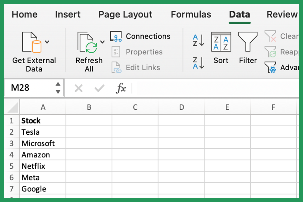
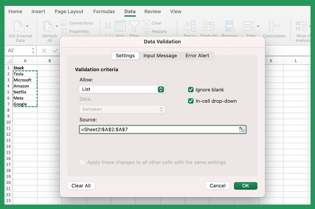
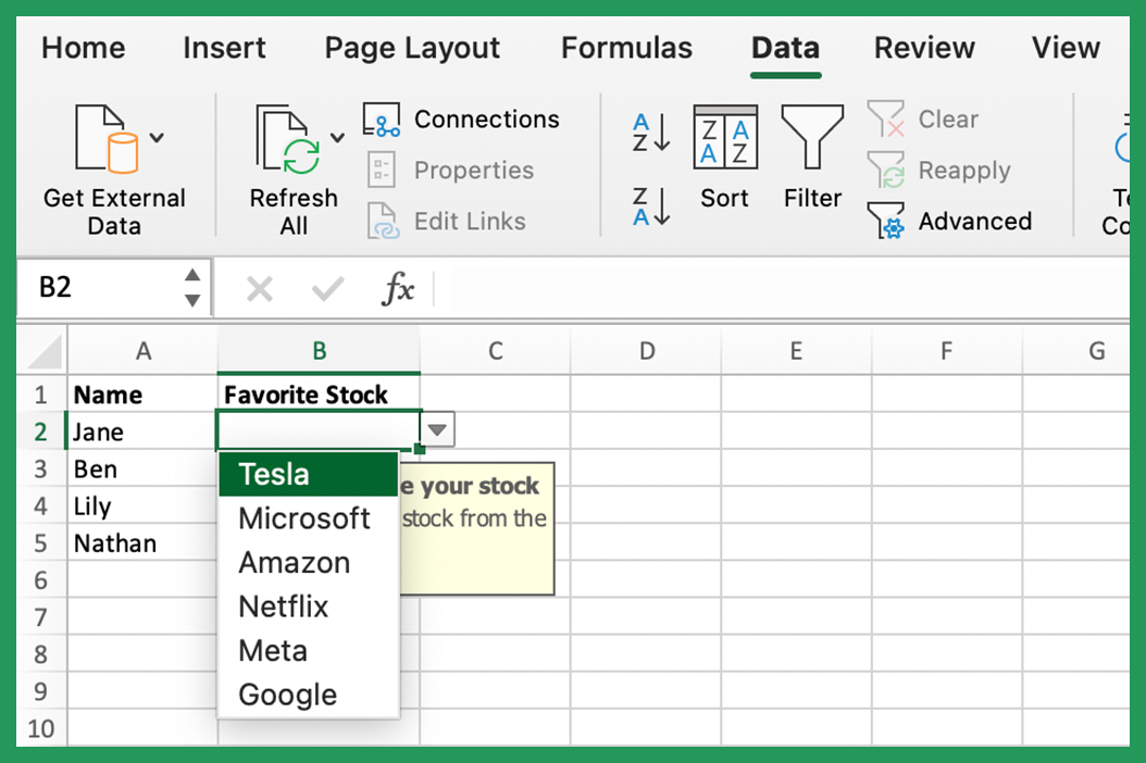
Next create a list of items that people are allowed to choose from, with no blank cells. I have given people the choice between, Tesla, Microsoft, Amazon, Netflix, Meta and Google. Ours are on Sheet2 in range A2:A7 in this case.
Back in our first worksheet, select cell 'B2'. Then go to the data tab on the menu and in the data tools group section of the ribbon you will see 'Data Validation'.
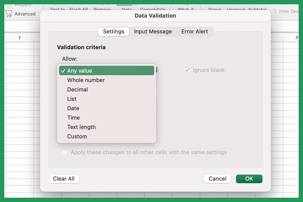
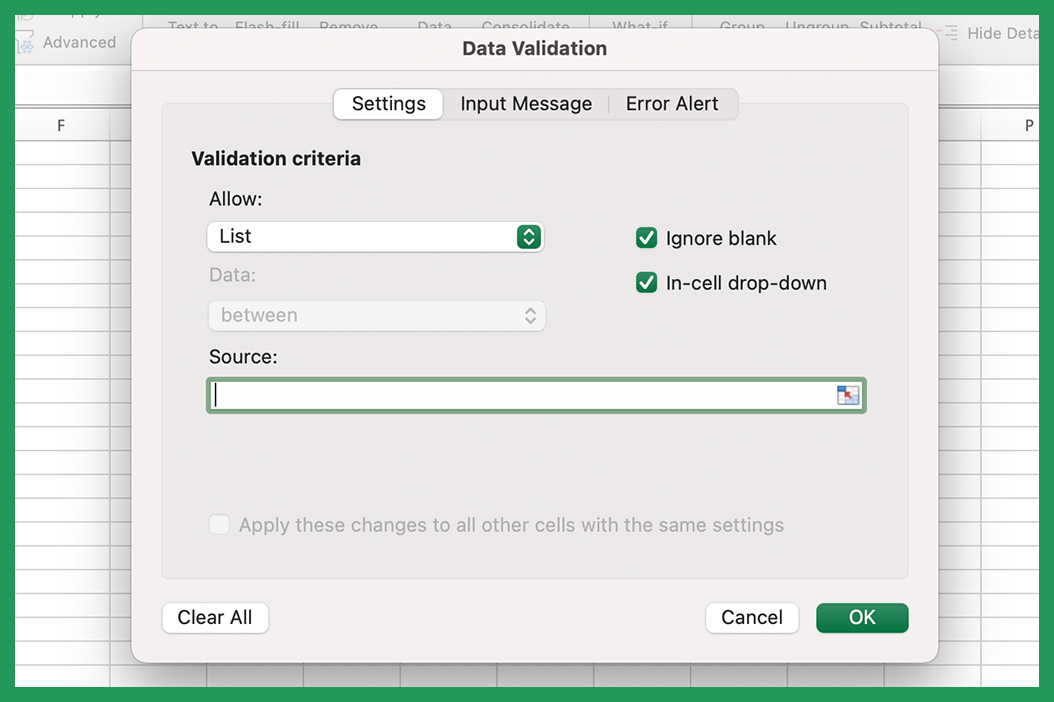
We will be presented with the Data Validation dialog box. In the settings tab, under validation criteria, in the Allow box, select list.
Next put your cursor in the source box, the data here can be entered into the source field in a couple of ways.
Click on the second worksheet we created without closing the modal and highlight the range of cells we want people to be able to choose from. To add a new item to the list when it is on a second sheet, you can add a list item below the final item and update the range that the source is covering.
Note: To avoid having to manually update the source, you can insert a row by left clicking one of the existing items, pressing insert and selecting shift cells down. The new item you enter should automatically be covered by the source range, but it is always worth double checking.
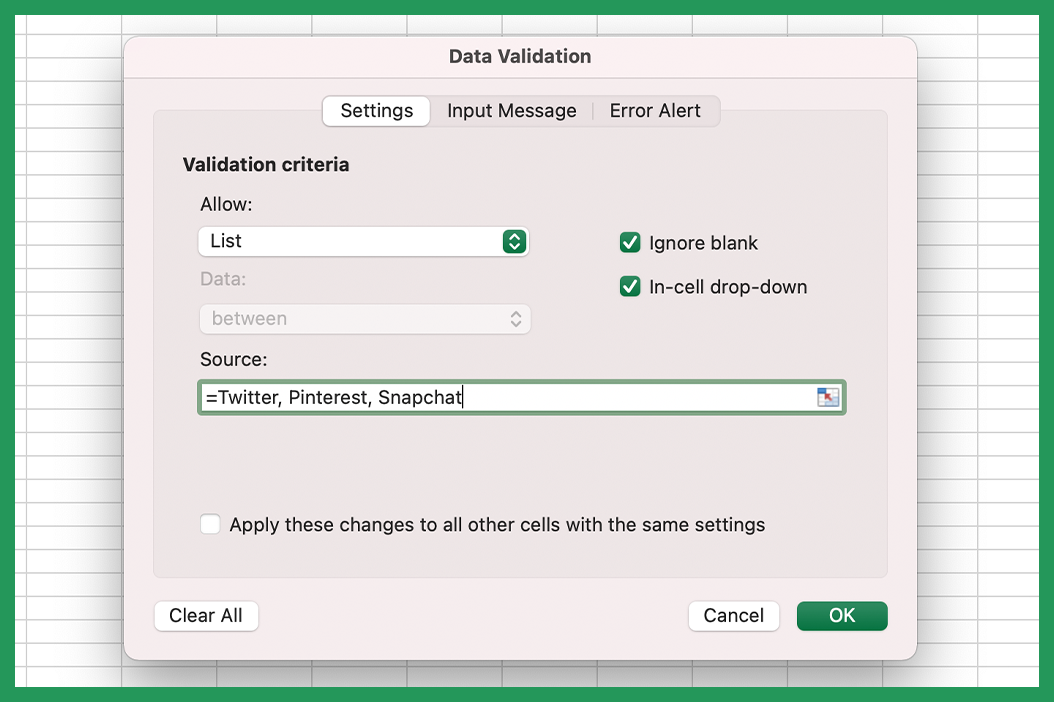
Alternatively, it can be entered as a comma separated list. If you wish to add a new item to the list it can simply be added to the end of the list after a comma.
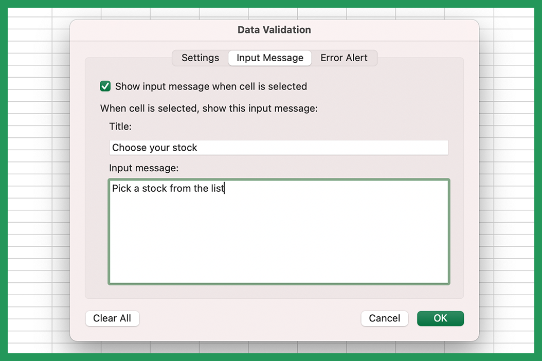
Move to the Input Message Tab and add a title and input message if you wish.
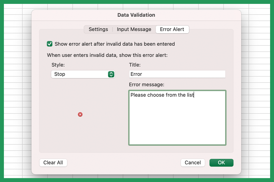
Finally, in the Error Alert tab, make sure 'show error alert' is ticked. We want to the only options to be the ones on the list and we will show a helpful message if something else is entered. If 'show error alert' is ticked and we don't enter a message, it will default to the excel warning.
Hit 'OK' and our drop down will appear. You will see that input message we entered above helps guide the user. Note: You may need to click on the cell to see the dropdown.
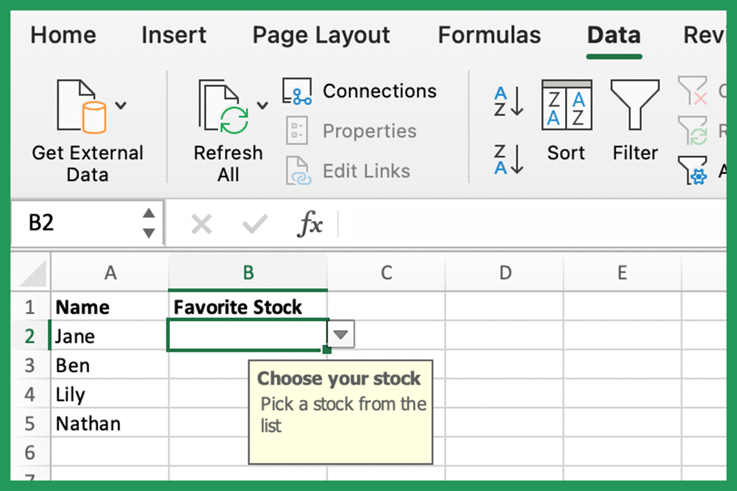
Your drop-down list is now created! To use it, simply click on the down arrow next to the cell and select the desired value from the list. In order to see the arrow, you must be in cell B2 in this example.
We can then drag the cell to cover all of the names so each person can make their choice.
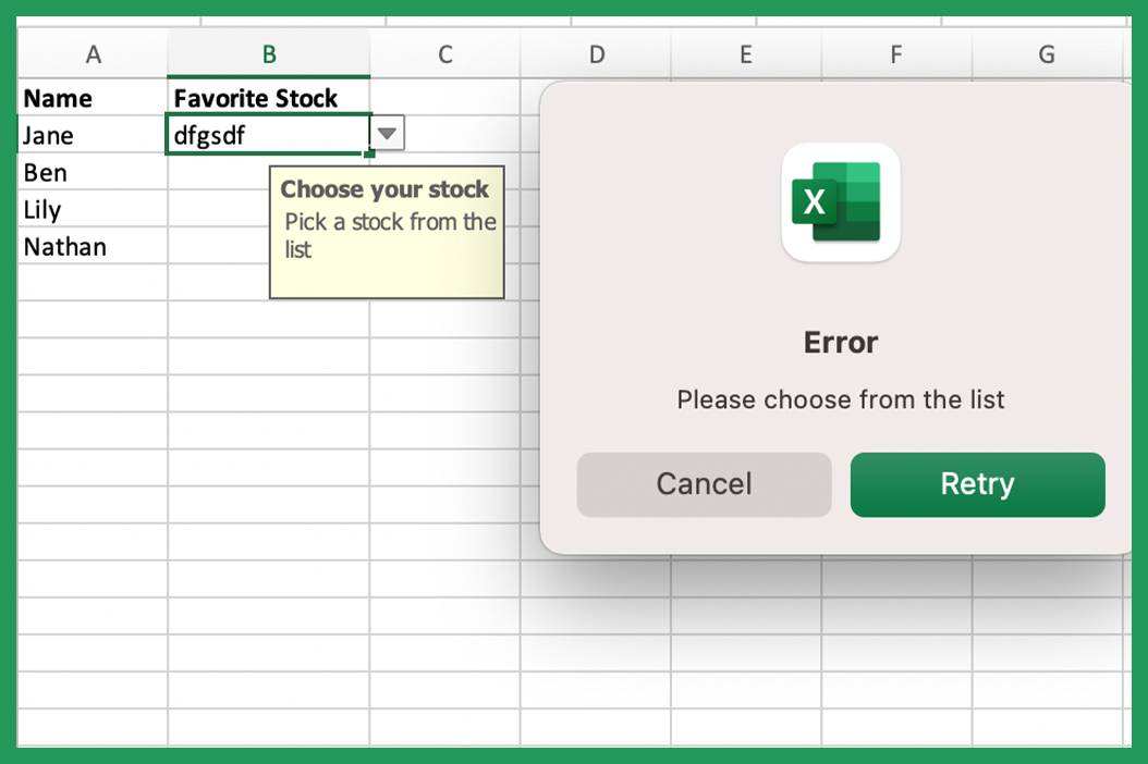
If we enter invalid data, the error message that we created earlier will show and give us the option to retry.
3. How To Remove A Drop Down List
If you want to remove a drop down without deleting the data:
1. Select the cells that contain the drop down list.
2. On the Data tab, click Data Validation.
3. Click Clear All.
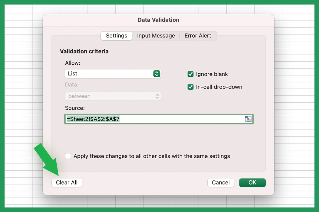
4. Click OK.
Your drop down list should now be removed.
Note:
- If you would prefer to use a named range, you can highlight the values you would like in the range and then create a name for the group of cells in the name box and reference it in the source box. You will need to go into name manager to update this range.
- Additionally you can use the offset function (=OFFSET(reference, rows, cols, [height], [width])) to reference the list to make it dynamic drop down list.
- The UNIQUE function can be used to ensure no duplicate values are included in your array.