HLOOKUP stands for 'Horizontal Lookup'. It is used for looking up the value of a cell in a table or array of data. The function looks left to right across the row of a table or array, and returns the value in the specified column.
The best use of this function is when your lookup value is in the top row of the table and your desired value is in the same column but in the lower rows.
Here is HLOOKUP function and its parameters:

This syntax may appear intimidating at first, but we'll start with an example to demonstrate how simple these frightening-looking parameters are when broken down.
Product Data - Example #1
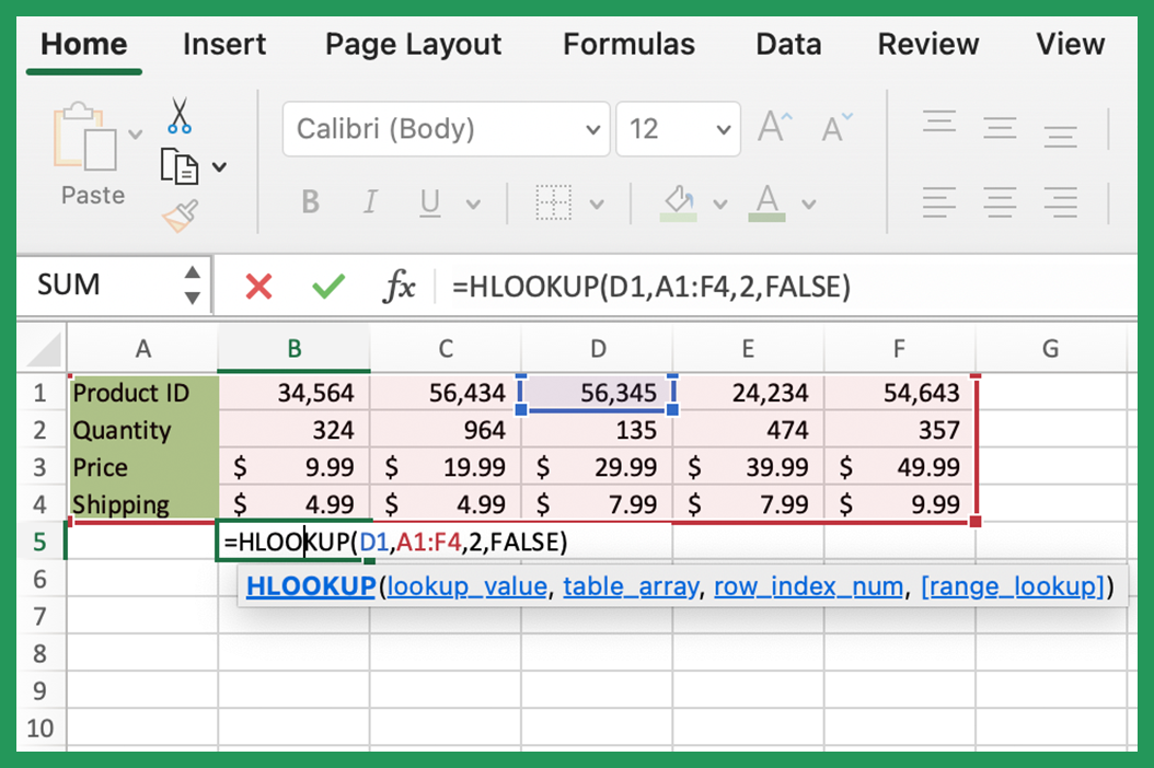
Here is a set of product data, detailing, price, quantity, and shipping cost. How could we use the HLOOKUP formula to find out how many mops this retailer has left in stock?
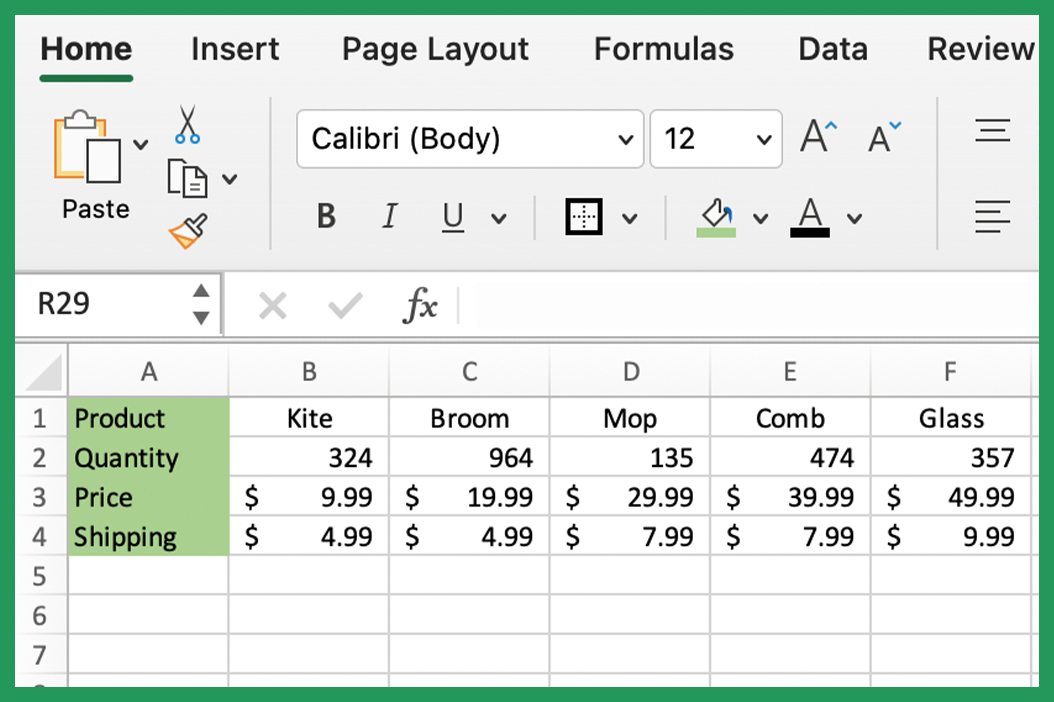
Here is the data if you would like to follow along with the example on your .
| Product | Kite | Broom | Mop | Comb | Glass |
|---|---|---|---|---|---|
| Quantity | 324 | 964 | 135 | 474 | 357 |
| Price | $9.99 | $19.99 | $29.99 | $39.99 | $49.99 |
| Shipping | $4.99 | $4.99 | $7.99 | $7.99 | $9.99 |
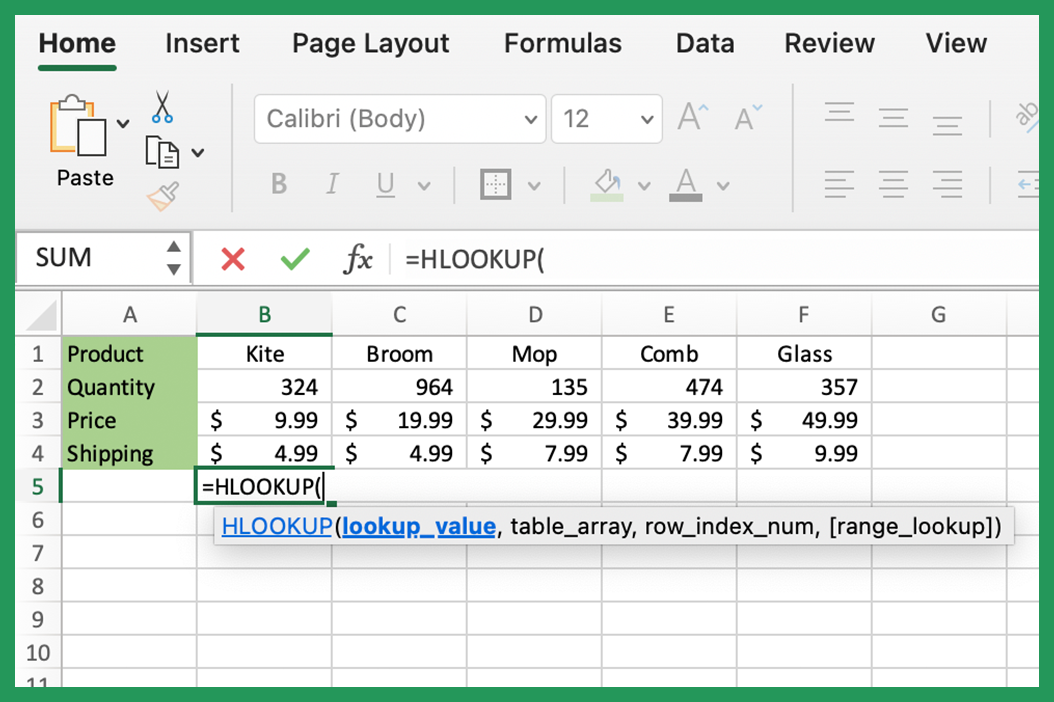
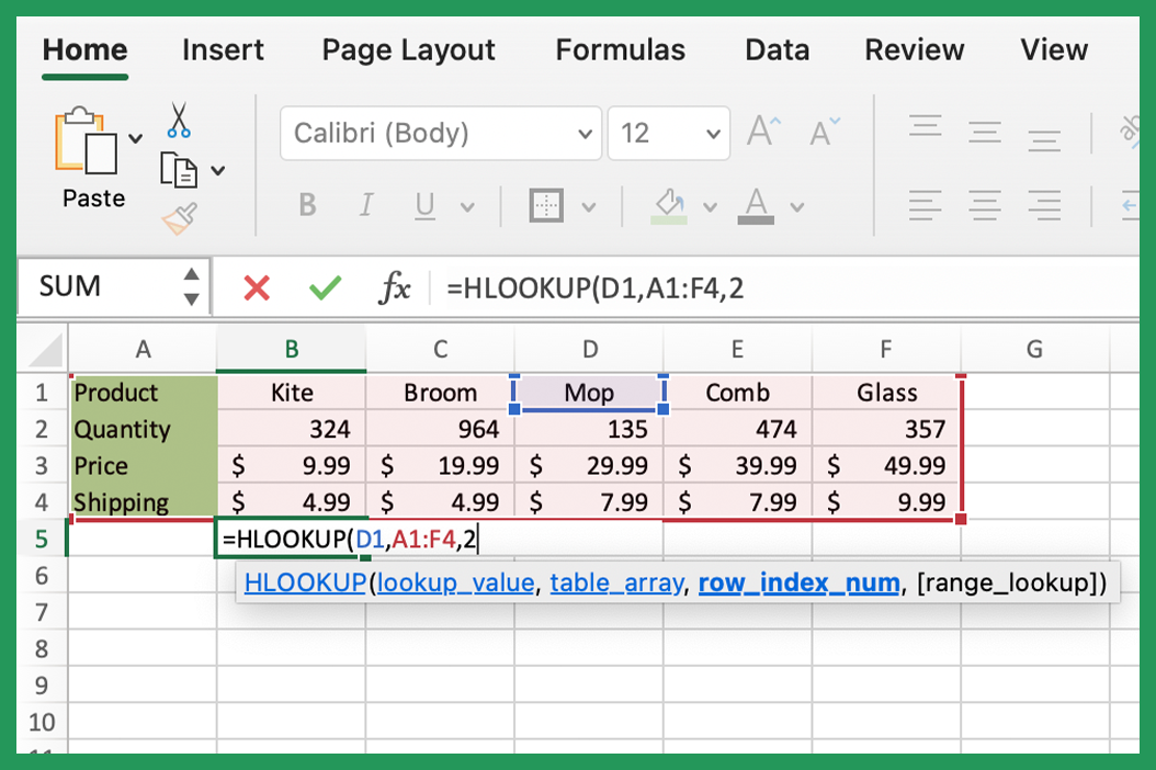
- Start with the function, =HLOOKUP( and then Excels assistant will let us know what parameters it needs.
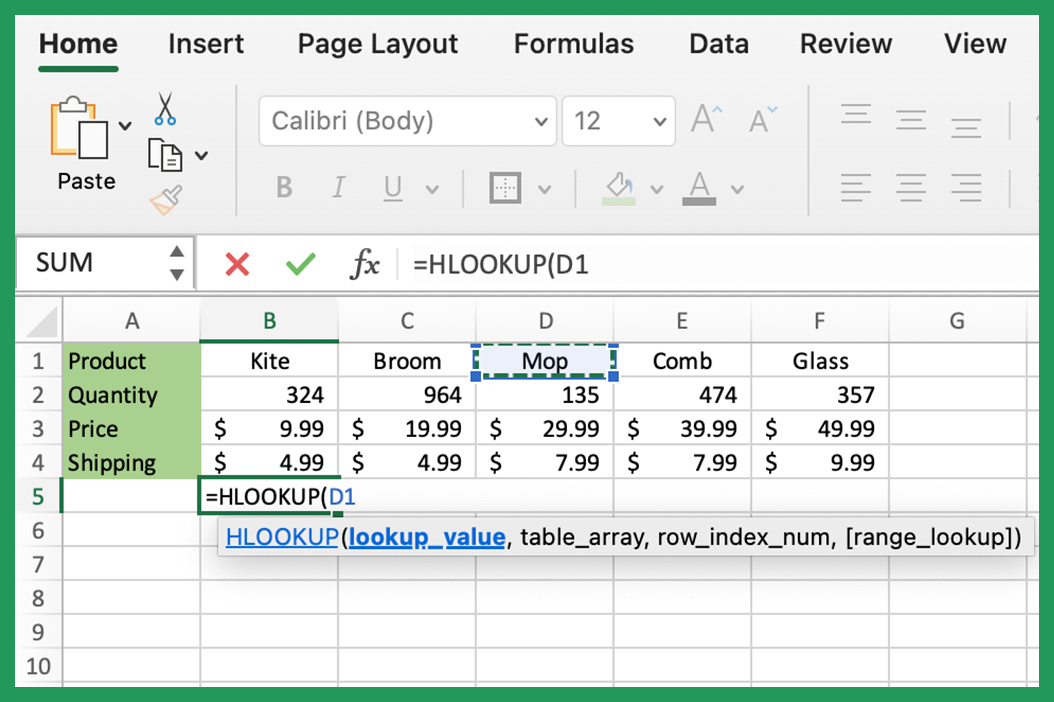
- The value we want to check is for the mop and that is located in column D and row 1 so we enter that as the lookup value.
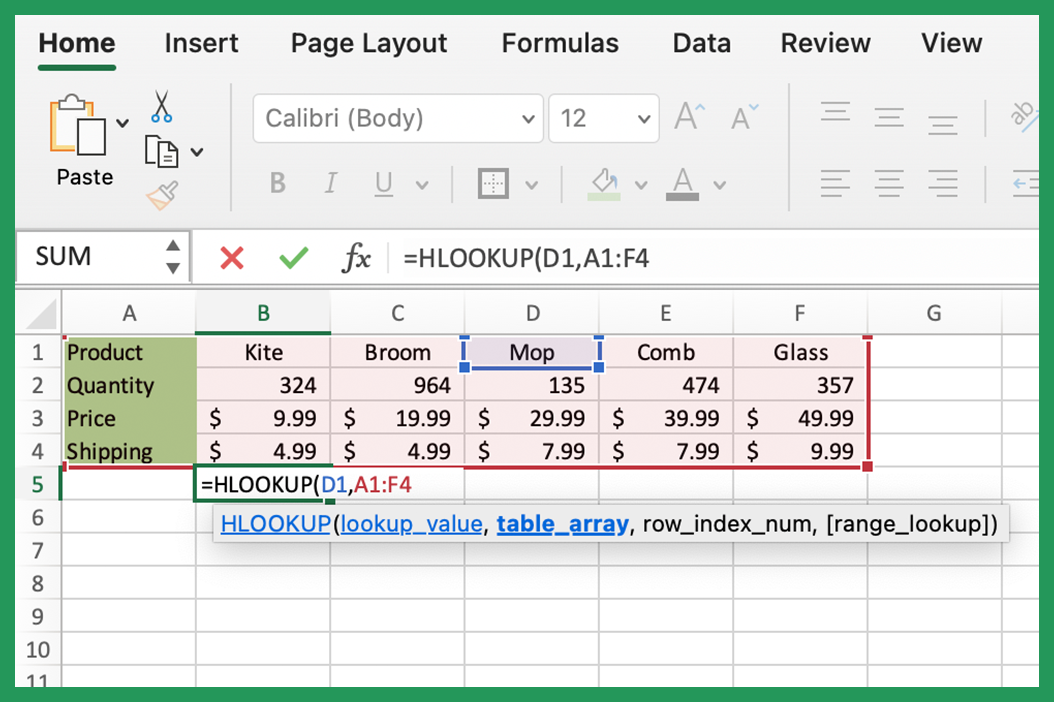
- The table we are searching is located between cell A1 and f4, so we enter them for the table array separated by a colon.
- Next we choose the row that we want the function to search in, for our example we want to find the quantity which is in row 1, so that is the third argument we enter.
- Finally we decide whether we want an exact or approximate one. In our case, we want an exact match so enter FALSE.
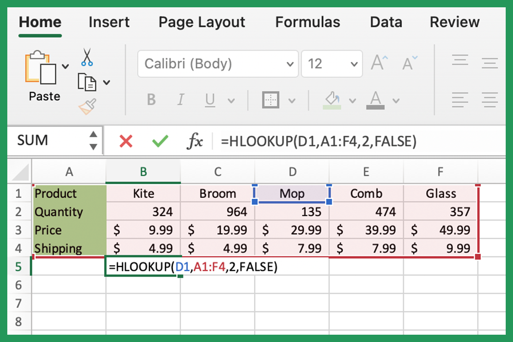
- Finally, hit enter and it will calculate the result.
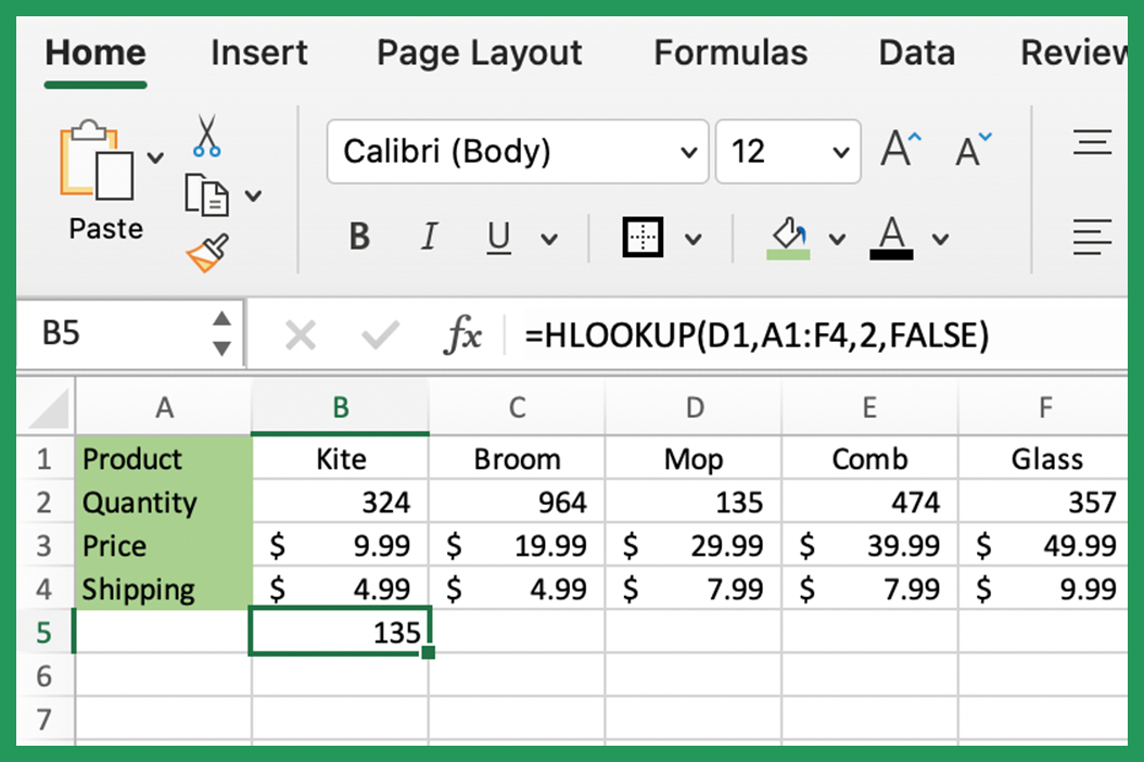
The answer is 135! We can confirm this is correct by manually looking at the quantity of mops in cell D2.
More details about the argument of the HLOOKUP function:
- Lookup_value (required) – the value you want to look up in the first row of the table.
- Table_array (required) – The table that is being searched. It must contain at least two rows of data, including the first row that will be searched for the value we are looking up. This gives the function the range within which it can find your value and return it. IMPORTANT: the data in the table should be sorted into ascending order when the range_lookup is TRUE otherwise an incorrect result may be returned.
- Row_index_num (required) – The row number within the table which will be searched to find and return the matching value. If the row number input is less than 1 a #VALUE error will be returned and if the row number is larger than the number of rows in the table a #REF! error will be returned.
- Range_lookup (optional) – If you enter TRUE or omit this argument, an approximate match is returned; if you enter FALSE, an exact match is returned. By leaving it blank or entering TRUE, an approximate match will be a satisfactory result (i.e. if the exact match is not found an approximate match will be accepted and returned). However, if FALSE and an exact match is not found, the #N/A error will be returned.
Further Examples
For the lookup_value parameter you can use a number or string, or reference a cell that contains a number or a string.
String Example =HLOOKUP(“example”,C1:E4,2,0) – looking for the string “example” in the table C1:E4 and the return value will be from the second row.
Number Example =HLOOKUP(1202,C1:E4,2,0) – looking for the value 1202 and returns a value from the second row (1200).
Cell Example =HLOOKUP(A1,C1:E4,2,0) – looking for the value from cell A1 and returns a value from the second row. If you are going to copy the function it can sometimes be necessary to use the absolute reference. In this case, the absolute reference for the lookup_value would be $A$1.
Your table_array can live on either the worksheet you're working on or another separate worksheet in your workbook.
Same worksheet Example =HLOOKUP(“my_value”,C1:E4,2,0) – referencing a table in the range C1:E4.
Separate worksheet Example =HLOOKUP(“my_value”,worksheet_name!$C$1:E$4,2,0) – referencing a table on a sheet called "worksheet_name" in the range C1:E4.
- You can use any whole number for the row which is between 1 (less than 1 will return you #VALUE! as an error) and the total number of rows in your table (otherwise HLOOKUP function can return you #REF as a value):
Same Row =HLOOKUP(“my_value”,C1:E4,1,0) – looking for the value in the first row. This search returns you the same value you used for lookup – “my_value”.
Second Row =HLOOKUP(“my_value”,C1:E4,2,0) – looking for the value in the second row, returns “hlookup_value”.
Eighth Row =HLOOKUP(“my_value”,C1:E4,8,0) – This would return a #REF error as there are not eight rows in this particular table.
Generally I use FALSE for the fourth parameter as I generally am looking for a specific value, and therefore want exact matches. There are cases where TRUE can be useful such as a list of names where some are start with a capital letter and others don't. It's very important to be careful with this fourth parameter.
By default, MS Excel uses TRUE (or 1) for this argument if you do not specify it (it is an optional parameter) and performs an approximate search.
It’s always very important to check this argument to get the right values. For exact matches use FALSE (or 0) as the fourth parameter.
Using 0 =HLOOKUP(“sweater”,C1:E4,2,0) looks for return value corresponding to “jumpers” and looks for an exact match
Using FALSE =HLOOKUP(“sweater”,C1:E4,2,FALSE) – also looks for return value corresponding to “jumpers” and looks for an exact match, it is just a different way or writing the same function.
Errors When Using HLOOKUP
- #N/A – occurs when lookup_value is not available in the first row of the table.
- #REF – error in the row_index_num argument. Have a look at your table and check the range is correct.
- #VALUE – also wrong number for the row_index_num, but when you use less than 1 as this parameter.
Note: IFERROR works well to ensure a certain action occurs when an error is returned.
- Not using absolute referencing ($) when copying a formula to the other cells. It’s a common problem and you can fix it fast. Just press F4 or add $ signs to the reference of a table, like in the example:
=HLOOKUP(“my_value”,$C$1:$E$4,2,0)
Note: It's good practice is to add absolute references to the Table_array argument when you use HLOOKUP and VLOOKUP functions.
HLOOKUP function with wildcards
This function can become even more powerful with wildcards. You can use these symbols in the first argument (lookup_value) to find information based on part of some text in the cells:
- ? (question mark) – to match a single character
- * (asterisk) – to match a sequence of characters
Note: If you want to perform a vertical lookup – use VLOOKUP function. Also, you can use a new improved function (XLOOKUP). It’s easier than using both HLOOKUP and VLOOKUP and it works in any direction.