Guide To Using INDEX MATCH EXCEL

What Are INDEX and MATCH Functions?

The INDEX and MATCH function is an excellent tool for looking up Excel values. It's a flexible and powerful formula that can be used for a variety of tasks. This guide will show you how to use the INDEX MATCH formula in Microsoft Office Excel.

The INDEX MATCH Formula combines two functions: INDEX and MATCH in Excel.

=INDEX() generates the value of a cell in a table based on the column and row number.

=MATCH() generates data on the position of a cell in a row or column.

The two formulas in combination can find and return the data or value of a cell in a table which is based on vertical and horizontal criteria.

For example, in the corporate world, you can use the INDEX MATCH formula to look up a customer's name based on their customer ID. Or, you can use it to look up an employee's salary based on their employee ID.

You'll need a populated table and a lookup value to use the INDEX MATCH formula. The table of data can be in any shape or form, with multiple criteria, but it must have at least one column and one row. The lookup value can be a number, text, or even another formula.

Once you have your data and lookup value, you can start using the INDEX MATCH function. The first step is to create an index column. This column will be used for the lookup value in the table. Simply enter =INDEX(data, row, column) to do this.

Next, you'll need to create a MATCH column. This column will tell Excel which value to look up in the index column. To do this, enter the MATCH formula: =MATCH(lookup value, index column, 0).

Finally, you can use index and MATCH functions to look up the values in your table. Simply enter the formula: =INDEX(data, MATCH(lookup value, index column, 0), column).

With the INDEX and MATCH functions, you can quickly and efficiently find values in your Excel source data. This is essential for anyone who needs to work with large excel data sets.

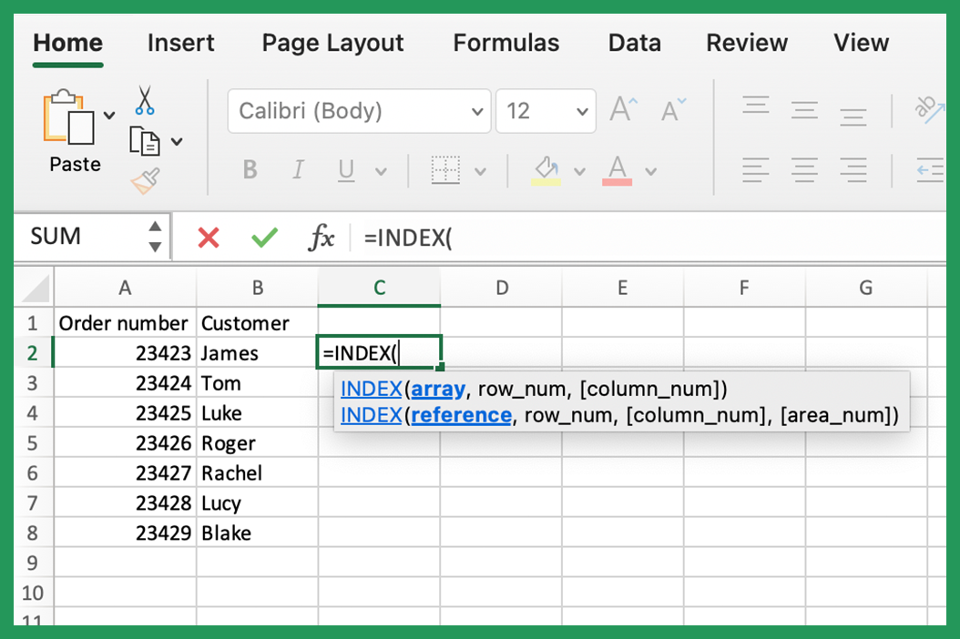
How to Use the INDEX Formula

Below is a table that we will use to demonstrate the INDEX function.

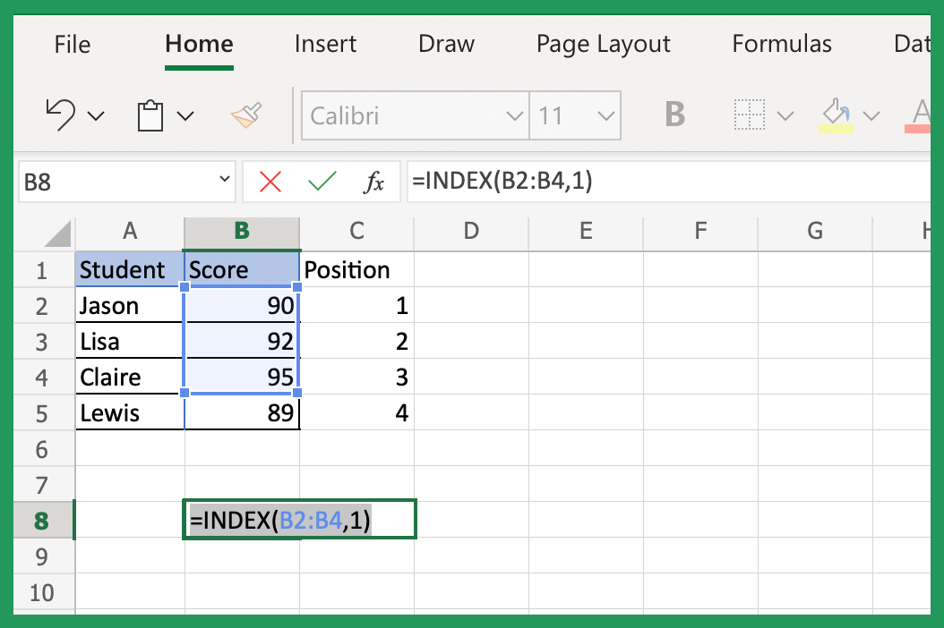
As you can see, this table has three columns: name, score, and position. We want to use INDEX to look up the score of the first person. In other words, we want to determine what grade Claire got on the test.

To do this, we will use the following formula: =INDEX(B2:B5,1).

The first data set is the range of cells that contains the scores (B2:B5). The second set is the cell's row number that contains the score we are looking for (1).

This formula returns 95, which is the score of the person in the first row.

Let's say we want to find out what position "Jason" is in. We can use the formula: =INDEX(C2:C11,5).

The first data set is the range of cells that contains the positions (C2:C11). The second set is the cell's row number that contains the position we are looking for (5).

This formula will return 3, Jason's position in the standings.

INDEX is a valuable tool for lookup values in a table. However, it has certain limitations. For example, what if we want to find Jason's score but don't know his position? We can use the MATCH function to help us out. We have more examples on this later!

How The Index Formula Works

INDEX returns a value from an ARRAY formula based on a given index number.

The syntax for INDEX is as follows:

INDEX(array, index_num)

Where "ARRAY" is the range of cells you want to browse through, and "index_num" is the number of cells in that ARRAY formula that contains the value you wish to return if you don't wish to include all the cells.

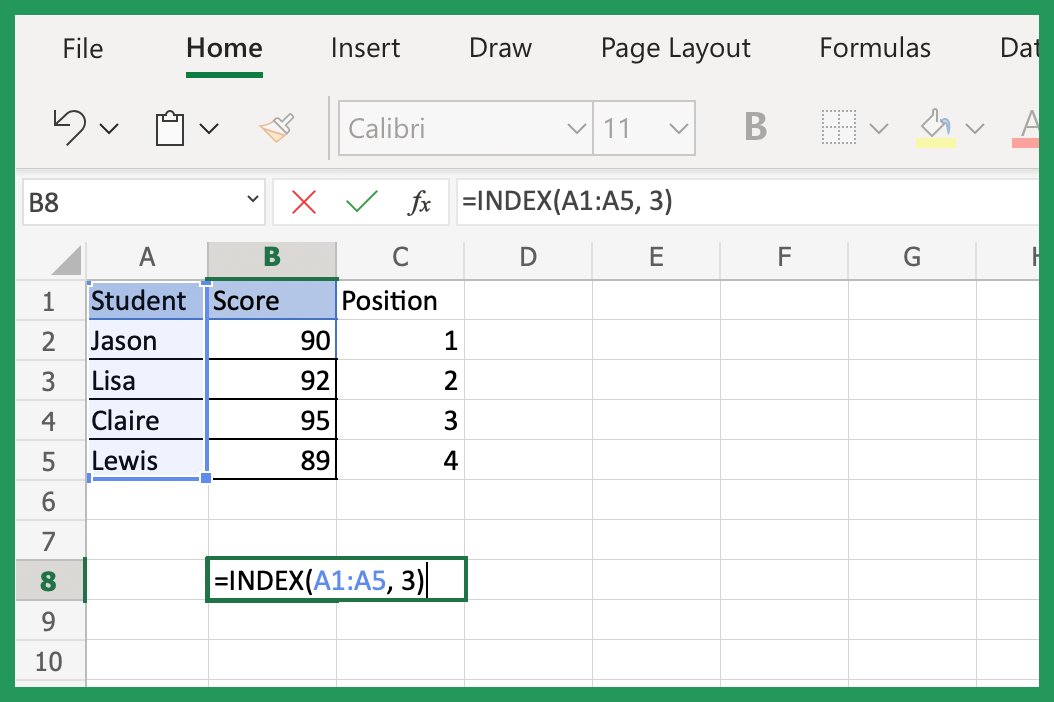
For example, if you have a list of names in column A and you want to return the name in cell A3, you would use the formula below:

=INDEX(A1:A5, 3)

MATCH returns the position of a given value in an ARRAY formula.

The syntax for the MATCH function is as follows:

MATCH(lookup_value, lookup_array, match_type)

Where "lookup_value" is what you're looking for, "lookup_array" is the range of cells where you want to look for that value, and "match_type" is an optional first argument that specifies how Excel should match the lookup_value with instances in the lookup_array. If omitted, Excel will use a "0" match type, which means it will find the first instance equal to the lookup_value.

You can use MATCH to return the position of a value in a sorted list.

To do this, you need to specify the sorted list as the ARRAY and use 1 as the MATCH type.

For example, let's say we have a list of numbers in ascending order, and we want to find the position of the number 9.

We can use the formula: =MATCH(9,A2:A11,1)

You are also able to work in descending order in more examples.

INDEX Function Syntax

Here is a simple description of each parameter:

• array - the range of cells that contains the data you want to look at
• uprow_num - the row number in ARRAY from which the value will be returned
• column_num - the column number in ARRAY from which the value will be returned

If you want to find a value based on multiple criteria, you can do so by combining the INDEX and MATCH functions.

How to Use the MATCH Function

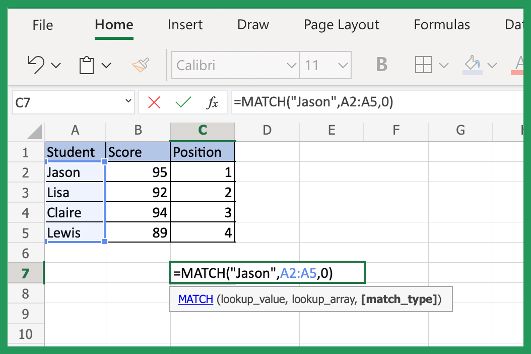
The MATCH function returns the exact position of a value in a table. So, for example, the formula =MATCH(95,C2:C5) would return 3, because 95 is the the third value in the table. In the first argument, we tell MATCH what we are looking for.

To do this, we'll use a formula like this: =MATCH("Jason",A2:A5,0). This formula will look in the range A2:A5 for the Jason's position in the table in the range C2:C5.

This formula will return 1, which is Jason's position.

As you can see, you can use the INDEX and MATCH functions together to look up instances in a table when you don't know the row numbers or even the column number.

You can also use the INDEX function to return multiple values without even knowing the column number!

Using Multiple Criteria Lookup

One of the more difficult lookups in Excel is based on multiple criteria. For example, you may have a list of employees and the department they work in. If you want to find the name of the employee who works in the Sales Department, you can use a simple VLOOKUP formula - usually for vertical lookups. But what if you also want to know the name of the employee who works in the Marketing Department? You need to use a lookup that allows for multiple criteria.

This is where INDEX and MATCH come in handy. With these two functions, you can create a multiple criteria lookup formula that will return the correct result, no matter which department you're looking up.

The INDEX function returns a value from an array based on a given index number, while MATCH returns the index number for a given value. By combining these two functions, we can create a multiple criteria lookup formula that is both flexible and powerful.

Two-way Lookup with INDEX and MATCH

You can use the INDEX MATCH formulas together to create a two-way lookup.

A two-way lookup is a lookup that returns a value from a table based on two criteria. (you can use ARRAY to return based on multiple criteria.)

For example, let's say we have a table with student names and test scores.

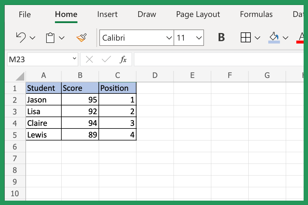
We want to be able to look up the name of the student who got the highest score on the test.

To do this, we can use the formula: =INDEX(A2:A5,MATCH(1,INDEX((B2:B5=MAX(B2:B5))*(A2:A5),0),0))

The INDEX MATCH formula above looks up the student's name who got the highest score on the test by using two-way lookup functions.

The first MATCH formula looks for the position of the number 1 in the ARRAY returned by INDEX.

INDEX returns an ARRAY of TRUE and FALSE that corresponds to whether each value in column B is equal to the maximum value in the same column.

The MAX function works to return the maximum value in B, which is 100.

So, the ARRAY returned by INDEX looks like this: {TRUE;FALSE;FALSE;FALSE;TRUE;FALSE;FALSE}.

The MATCH formula then returns the position of the first TRUE value in the lookup ARRAY, which is 1.

The MATCH formula is nested inside an INDEX, and it returns the student's name in row 1, column A.

The Left Lookup - Using INDEX and MATCH Instead of VLOOKUP

One of the key advantages of the INDEX MATCH formula over VLOOKUP function is that it can be used to look up instances in the leftmost column. This section explores the alternative to using VLOOKUP for a vertical lookup.

The VLOOKUP function can only look up instances to the right of the search column, which means the search column must always be the first column in the table ARRAY.

Using Left Lookup within INDEX and MATCH can find in any column in the table ARRAY, even if that column is to the left of the search column.

For example, suppose we want to determine which student scored 97 marks.

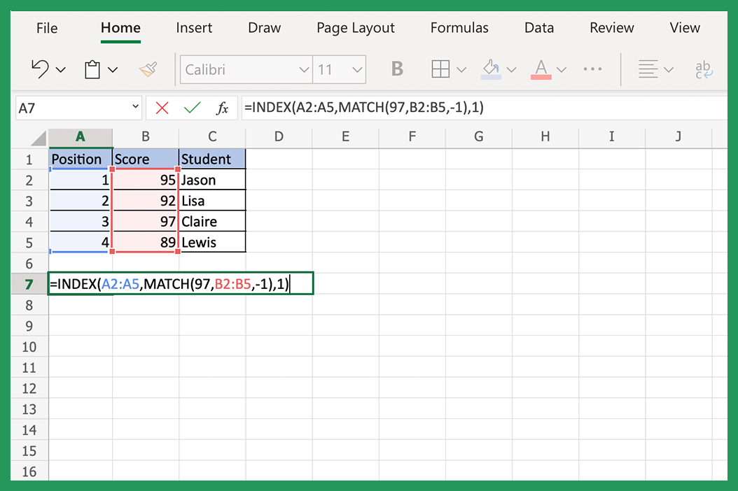
In this case, we'll use a formula with a reverse MATCH formula:

=INDEX(A2:A5,MATCH(97,B2:B5,-1),1)

The MATCH formula returns the position of 97 in the range B2:B7, and since we've used the -1 parameter, it returns the position of 97 from the bottom up.

This means it returns 2, because 97 is the 2nd value when you count from the bottom up.

The INDEX function then uses this row number to return the corresponding value in column A.

Index and match can also be used together to find an approximate match.

For example, suppose we want to find out which student scored closest to 95 marks.

To do this, we can use the formula:

=INDEX(A2:A11,MATCH(95,B2:B11,1))

This formula will return the name of the student who scored closest to 95.

Note that the "1" in the MATCH formula is important.

It tells Excel to find an exact match. If you omit the "1", Excel will find the closest match, which may not be what you want.

You can also use the INDEX MATCH formula to lookup values to the right of the search column.

To do this, simply switch the position of the lookup value and search column in the INDEX and MATCH formula.

If we wanted to lookup student names based on their marks, we could use the formula:

=INDEX(B2:B11,MATCH(A2,A2:A11,0))

This would return the name of the student who scored closest to 95.

You can also use the INDEX MATCH function with multiple criteria.

To do this, you need to use a lookup ARRAY. This formula performs calculations on more than one cell at a time.

Suppose we wanted to find the name of the student who scored closest to 95 marks and also had an attendance score of 80 or more.

We could use the following INDEX MATCH formula:

=INDEX(B2:B11,MATCH(1,(ABS(A2:A11-95)+(C2:C11<80)),0))

This would return the name of the student who scored closest to 95 marks and had an attendance score of 80 or more.

Using Case-sensitive Lookup Function

The MATCH function is not case-sensitive alone. However, you can use the INDEX MATCH formula to perform a case-sensitive lookup. For example, suppose we had the following table:

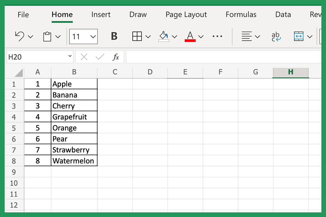
If we wanted to find the position of the word "orange" in column B, we could use the following INDEX MATCH formula:

=MATCH(INDEX(B1:B8,MATCH("orange",B1:B8,0)),B1:B8)

This would return value 5, since "orange" is the fifth item in B.

The INDEX MATCH formulas are used together to perform advanced lookups in Excel. INDEX returns a cell reference in a range based on its row and column numbers, and MATCH returns the row or column number of a cell in a range based on its value.

Using Closest Match Formula Correctly

Another example that showcases the flexibility of INDEX MATCH is the problem of finding the closest match. Suppose you have a list of numbers in column A and you want to find the closest match to a number in column B. Given the information below, we want to find the closest match for the number 50 in column B.

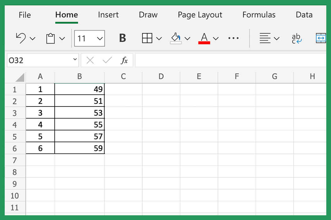
INDEX can return the value in any row from column A, but only if we give it the row number. MATCH can give us the row number of a value in the same column, but only if the value exists somewhere in that column. So how do we use these together to get the closest match?

We use INDEX and MATCH together like this:

=INDEX(A1:A6,MATCH(B1,A1:A6,1))

This returns a result in row 1, column A.

The MATCH function looks for the value 50 in column A and returns the row number where it finds that value. In this case, it's row 2. INDEX then uses that row number to return the value from column A.

If we change the number in column B to 51, MATCH finds a different result:

=INDEX(A1:A6,MATCH(B1,A1:A6,1))

This time, the MATCH function can't find the value 51 in column A, so it returns the row number of the next lowest value, 3. INDEX returns the cell from that same row in the same column. This can be expanded into more columns such as column C, column D.

How To Use MATCH for Exact Match Finds

You can use the MATCH function with the optional third argument if you want to find an exact MATCH. The third argument tells Excel how to MATCH the lookup value. If you set it to 0, Excel will find an exact MATCH. If you set it to 1, Excel will find the largest value that is less than or equal to the lookup value. The default is 1, so if you omit this last argument, Excel will look for an approximate MATCH instead of the largest value (you can also do the same to find the smallest value).

Let's say we have a list of numbers in column A and we want to find an exact MATCH for the number 50:

=MATCH(50,A1:A6,0)

This time, the MATCH function will return 4, because 50 is the fourth item in the list.

If we change the last argument to 1, Excel will look for an approximate MATCH and return 5, because 50 is less than 55:

=MATCH(50,A1:A6,1)

You can also use MATCH with the wildcard characters – ? and * – to find partial matches instead of just an approximate MATCH. For example, if we want to find a partial MATCH for the text "excel," we can use the formula below:

=MATCH("*excel*",A1:A6)

Also, MATCH finds the relative position of a cell in an ARRAY. For example, if we have the following ARRAY:

{1;2;3;4;5}

If we want to know the position of the number 3; we can use this formula:

=MATCH(3,{1;2;3;4;5},0)

The MATCH function works to return cell reference 3 because 3 is the third item in the ARRAY.