The Excel SUM function is a simple yet powerful tool for adding up data. It is used to add up a range of cells.
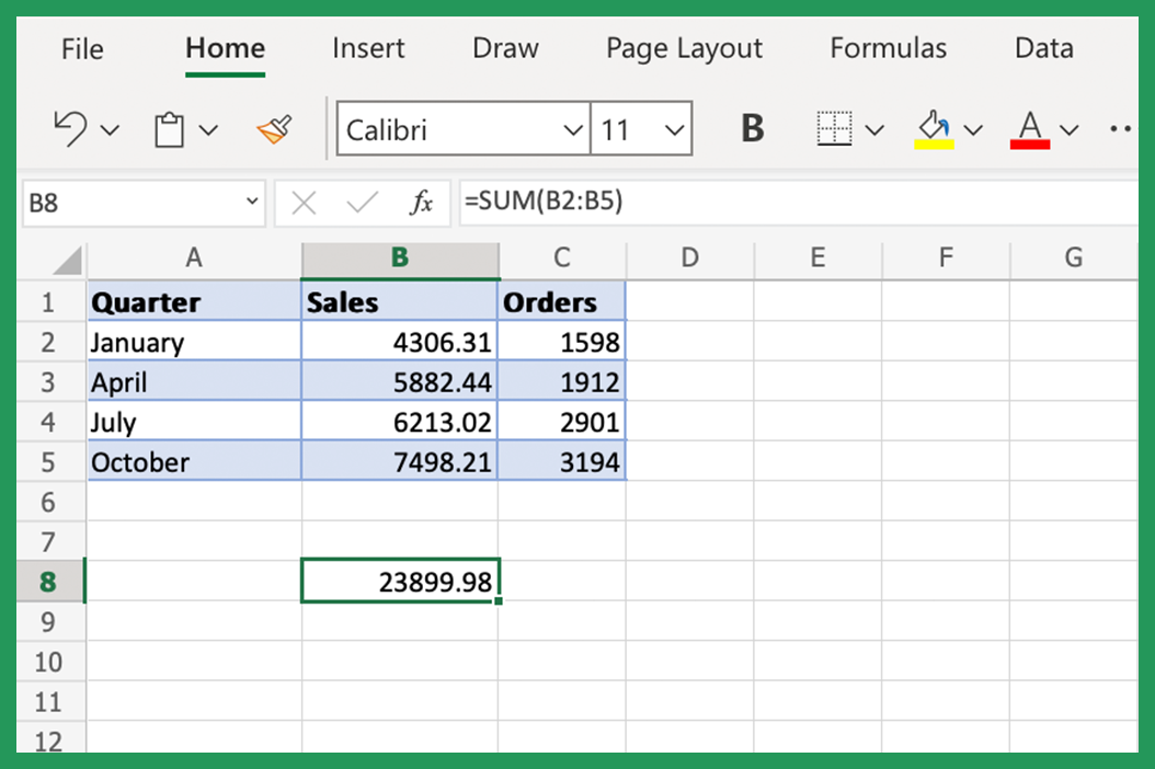
To use the SUM function, select the cell where you want the sum to appear and type =SUM( followed by the cell range you want to add up, separated by a comma. For example, to add up cells B2 through B5, you would type =SUM(B2:B5). Excel will then display the sum of the selected cells or a singular selected cell, as you can see below in our first example.
You can also use SUM to add up multiple cell ranges. For example, to add up cells A1 through A5 and B1 through B5, you would type =SUM(A1:A5,B1:B5). Excel will then display the sum of all of the selected cell data.
How Does the Excel SUM Function work?
The SUM function takes a range of cells as an argument. It then adds up all the cells in the range and returns the sum.
You can also use SUM to add up multiple cell ranges. For example, assume we have the following data in cells A1 through A5 and B1 through B5:
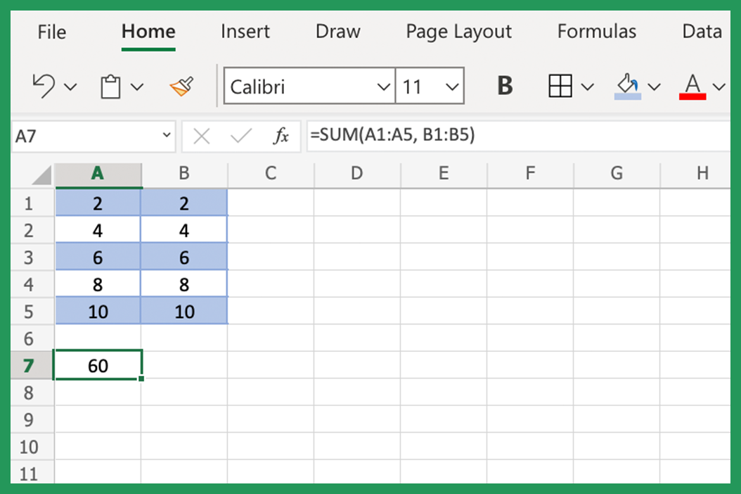
If we use SUM to add up this data using =SUM(A1:A5, B1:B5), Excel will return the sum of all the data, which is 60.
As you can see, the SUM function is a very versatile tool that can be used to add up data in a variety of ways.
What SUM Formula to Use?
You can use the following formulas to use the SUM function:
- The first way is to use SUM with a range of cells. For example, to add up cells A1 through A5, you would type the following SUM formula:
=SUM(A1:A5).
- The second way is to use SUM with multiple cell ranges. For example, to add up cells A1 through A5 and B1 through B5, you would type the following SUM formula:
=SUM(A1:A5,B1:B5).
Which way you use will depend on your data and what you want to do with it. Experiment with both ways to see which one works best for you.
Examples Using the Excel SUM Function
To see the SUM function in action, let's take a look at some examples.
Example 1: Adding Up an Entire Column of Data
Assume we have the following data in cells A1 through A5:
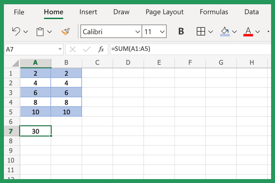
If we want to add up this data, we can use SUM. To do this, we would select cell A6 and type =SUM(A1:A5). Excel will then display the sum of the data in cells A1 through A5, which is 30.
Example 2: Adding Up a Row of Data
Assume we have the following data in cells A1 through E1:
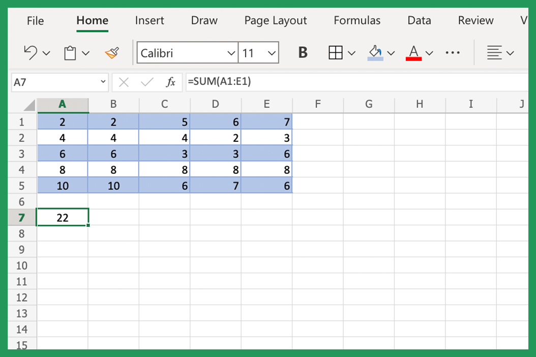
If we want to add up this data, we can once again use SUM. To do this, we would select cell F1 and type =SUM(A1:E1). Excel will then display the sum of the data in cells A1 through E1, which is 22.
Example 3: Adding Up a Range of Data
Assume we have the following data in cells A1 through C5:
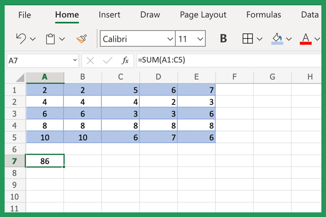
If we want to add up this data, we can use the Excel SUM function. To do this, we would select cell A7 and type =SUM(A1:C5). Excel will then display the sum of the data in cells A1 through C5, which is 86.
Example 4: Adding Up Multiple Cell Ranges
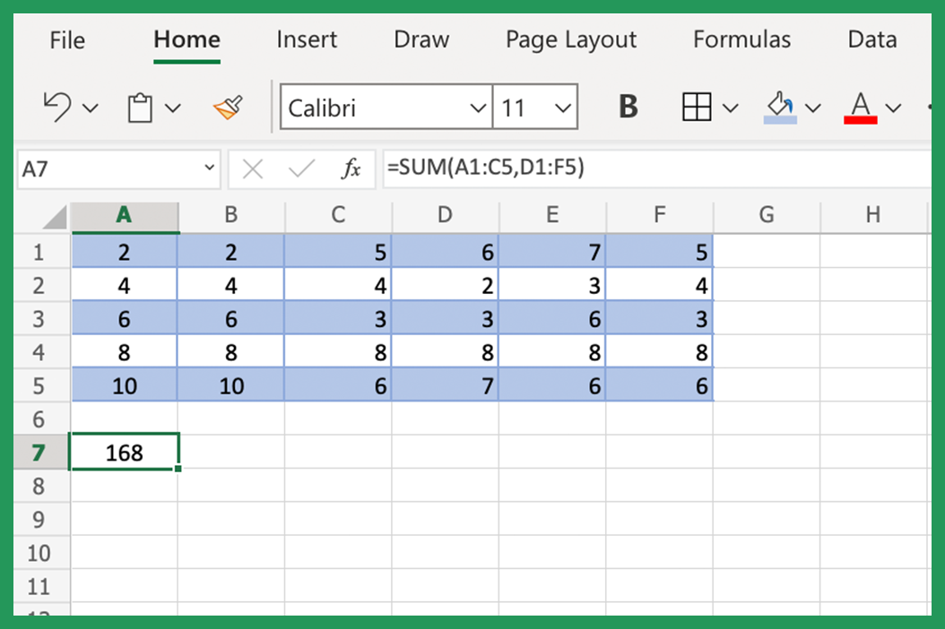
Assume we have the following Excel table containing data in cells A1 through C5 and D1 through F5:

If we want to add up this data, we can use SUM. To do this, we would select cell A7 and type =SUM(A1:C5,D1:F5). After you press Enter, Excel will then display the sum of the data in cells A1 through C5 and D1 through F5, which is 168 - as you can see in the screenshot above.
Excel SUM Keyboard Shortcut
You can also use a keyboard shortcut to add up data in Excel. To do this, select the values you want to sum and press Alt, press the plus sign (+) and the equals sign (=). Excel will then display the sum of the selected cells.
This keyboard shortcut is very handy if you want to quickly add up an entire column or row of data.
Using the Excel SUM Function with Other Functions
The SUM function can also be used in conjunction with other Excel functions. For example, you could use SUM to add up a column of data and then use the Excel AVERAGE function to calculate the average of the data.
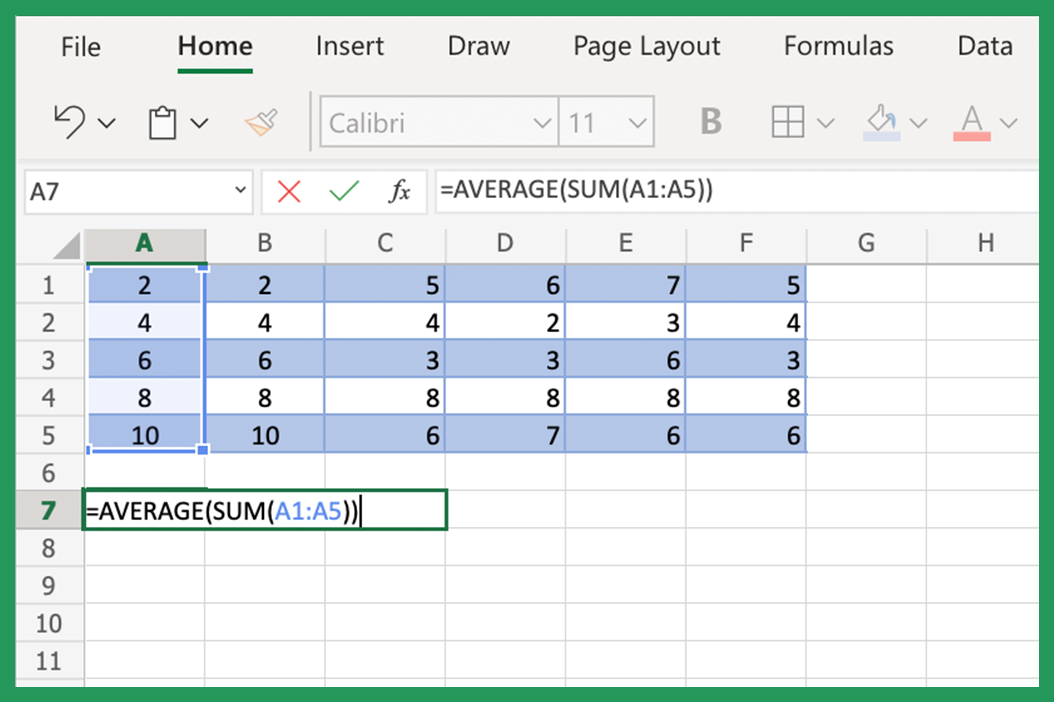
To do this, you would first select the cells you want to sum and then type =AVERAGE(SUM(A1:A5)). Excel will then calculate the sum of the data in values A1 through A5 and display the average.
You could also use SUM to add up an entire column of data and then use the Excel COUNT function to calculate the numeric value of cells that contain data.
To do this, you would first select the values you want to add up and then type =COUNT(SUM(A1:A5)). Excel will then calculate the sum of the data in cells A1 through A5 and display the numeric value of cells that contain data.
Using the SUM function the add Text Values of Filtered Data
The SUM function can be used to sum the data in filtered cells. This is useful if you want to sum only a subset of the data in a range. For example, you could use the Excel SUM function to sum only the data that meets certain criteria.
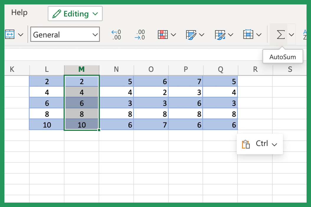
To use SUM to sum the data in filtered cells, follow these steps:
1. First, apply a filter to the data range.
2. Next, select the cells that you want to sum.
3. Finally, click the AutoSum command on the Excel ribbon.
Excel will then display the sum of the filtered data in the single cell next to the last cell in the selection.
Using the SUBTOTAL Function with SUM
You can even use the SUBTOTAL function to sum the data in filtered data. The SUBTOTAL function has the added benefit of being able to exclude hidden cells from the sum.
To use the SUBTOTAL function to sum the data in filtered data, the following formula shows you how:
“SUBTOTAL(function_num,ref1,ref2,…)”
As mentioned previously, the most convinient way is to double click AutoSum.
Using SUMIFS in Excel
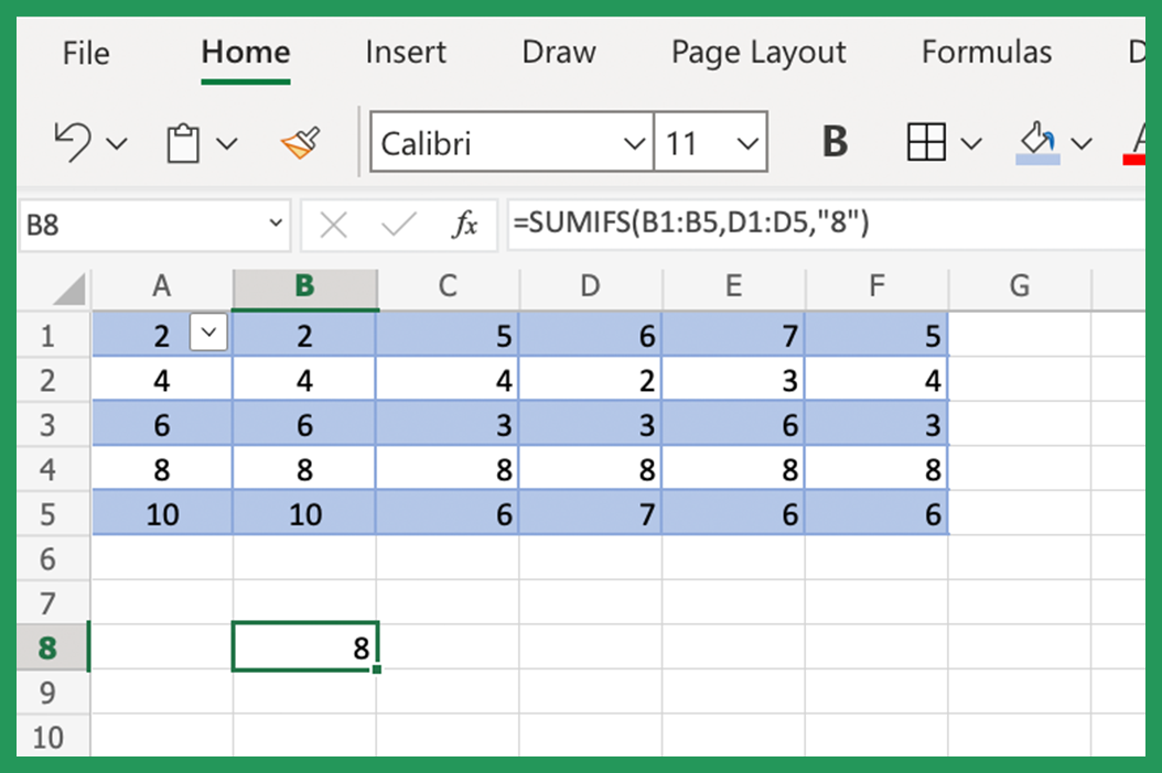
The Excel SUMIFS function is an Excel logical function that can be used to sum data based on multiple criteria.
The Excel SUMIFS function is pretty similar to the Excel SUMIF function, but it has the added ability to sum data based on multiple criteria. The Excel SUMIFS function formula is as follows:
“SUMIFS(sum_range,criteria_range1,criteria1,[criteria_range2,criteria2],…)”
On the other hand, the Excel SUMIF function can only be used to sum data based on a single criterion.
Using The SUM Excel Function with OFFSET
The Excel OFFSET function can be used to create a reference to a cell or range of cells that is relative to another cell. The OFFSET formula is as follows:
“OFFSET(reference,rows,cols,height,width)”
OFFSET has the following arguments:
reference - The cell or cell range that you want to base the offset on.
rows - The number of rows that you want the offset to be.
cols - The number of columns that you want the offset to be.
height - The height of the cell or referenced range.
width - The width of the cell or cell range that you want to reference.
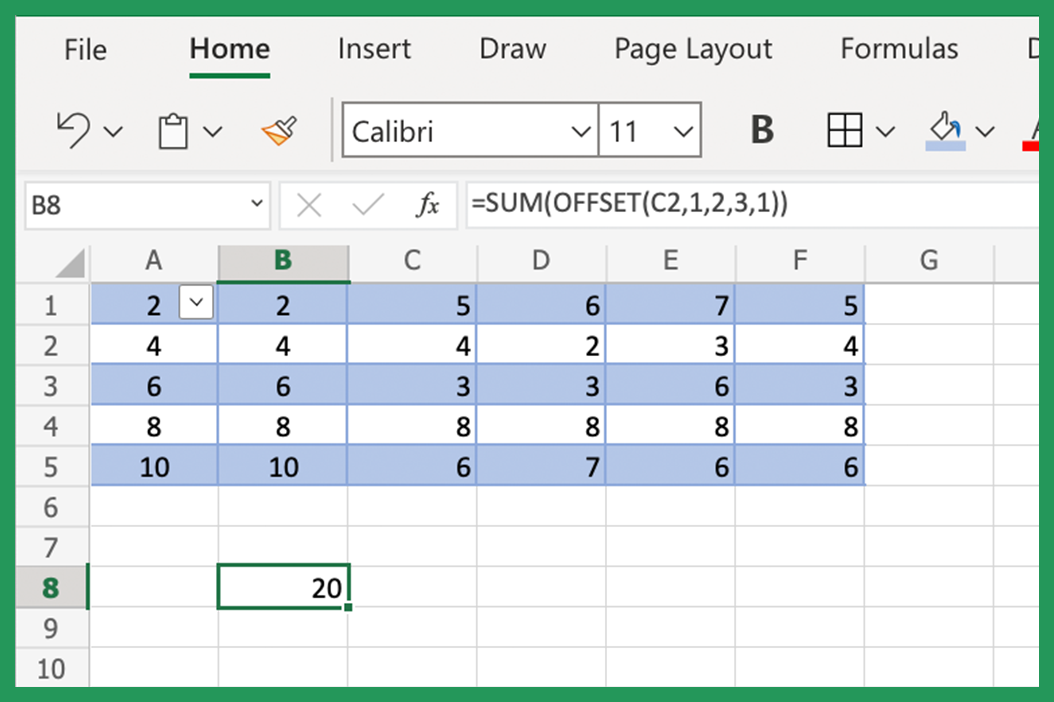
You can use OFFSET in conjunction with the SUM function to sum a range of cells that is a specified number of new rows and columns away from another cell or range of cells. For example, you could use the Excel OFFSET function to sum the range of visible cells that is 3 rows and 2 columns away from cell A1.
To use the Excel OFFSET function to sum a cell range or sum columns, follow these steps:
1. First, select the cell that you want to sum.
2. Next, click the Formulas tab on the Excel ribbon.
3. Then, click the Insert Function button.
4. Excel will then display the Insert Function dialog box.
5. In the Insert Function dialog box, select the SUM function.
6. Excel will then display the Function Arguments dialog box.
7. In the Function Arguments dialog box, enter the formula:
“SUM(OFFSET(A1,3,2))”
8. After you press Enter, Excel will sum the range of cells that is 3 rows and 2 columns away from cell A1.
That is how you sum a column or row in Excel!
SUM Function Errors
If the SUM function returns an error, it is most likely because:
- You have referenced a cell that contains text instead of numeric values.
- You have referenced a cell that contains a SUM formula that returns an error.
- You have referenced a cell that is blank.
What Are Cell References?
Cell references are a way to refer to a cell or cell range in Excel. Cell references are used in formulas to tell Excel which cells to use in the calculation.
There are two types of cell references to consider in Microsoft Excel: relative and absolute.
Relative cell references are a reference to cells that are relative to the position of the formula. Relative cell references change when the same formula is copied to another location.
Absolute cell references are references to cells that are not relative to the position of the formula. Absolute cell references don't change when an Excel formula is copied to another location.
Relative cell references are the default in Excel. This means that if you don’t specify an absolute or relative cell reference, Excel will assume you want relative cell references.
You can make a cell reference absolute by using the dollar sign ($) in front of the column letter and total row number. For example, the cell reference A$1 is an absolute reference to the first cell A1.
SUM Function Tips
Here are some tips for using the SUM function:
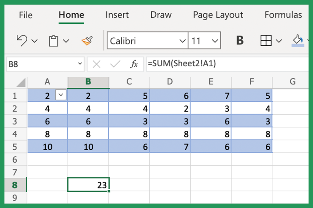
You can reference cells in other worksheets by using the sheet name followed by an exclamation mark (!). For example, to reference cell A1 on a sheet named Sheet2, you would use the following formula: =SUM(Sheet2!A1).
You can reference cells in other workbooks by using the workbook name followed by an exclamation mark (!). To reference cell A1 in a workbook named Workbook1.xlsx, you would use the following example: =SUM(Workbook1.xlsx!A1).
You can add up cells that are not next to each other by using the SUM function. For example, to add up cells A1, C1, and E1, you would use the following formula: =SUM(A1,C1,E1).
You can use SUM to quickly sum a total column or row of data by selecting the visible cells and then pressing Alt + =. Excel will then display the sum of the selected cells.
SUM Function Limitations
The SUM Excel function has the following limitations:
- You can only reference a maximum of 255 cells in a single SUM function.
- You cannot use an array constant (e.g. {1,2,3}) as one of the arguments for the SUM function.
There are a few things to keep in mind when using the SUM Excel function. First, you can only reference a maximum of 255 cells in a single SUM function. Second, you cannot use an array formula (e.g. {1,2,3}) as one of the arguments for the SUM function.
Finally, the SUM function will not automatically update if the text values in the cells it references change. This means that you will need to recalculate the SUM function manually if the values in the cells change.
Conclusion
As you can see, the SUM Excel function is a very versatile tool that can be used to add up data in a variety of ways. So next time you need to add up some data, don't reach for the calculator - reach for Excel and the SUM function!
The SUM function is a quick and easy way to add up data in Microsoft Excel. Give it a try the next time you need to sum a column of numeric values!