We'll explain what the axes are and why you might want to switch them. We'll also give you some tips on how to understand Microsoft Excel's chart axes.
Finally, we'll show you how to rearrange your data so that it specifies the axis that you want. Let's get started!
What The X and Y Axes Are
The x-axis is the horizontal axis on a graph, and is usually labeled with the independent variable. The y-axis is the vertical axis on a graph. It is usually labeled with the dependent variable. You might want to switch the axes so that the dependent variable is on x and the independent variable is on the y (two perpendicular lines). This can be helpful if you are trying to compare data sets that have different units of measurement.
For example, you might want to compare data that is measured in dollars with data that is measured in percent change. In this case, it would make more sense to put the dollar values on x and the percent change values on y.
Why You Might Want to Switch X and Y Axis in Excel
There are a few different reasons why you might want to literally swap the x and y-axis in Microsoft Excel. As we mentioned above, it can be helpful if you are trying to compare data sets that have different units of measurement. It can also be helpful if you want to make sure that your data is displayed in the order that you want.
For example, if you are trying to compare data from different years, you might want to put the most recent year on the x-axis and the earliest year on the y-axis. This will ensure that your data is displayed in the correct order.
Explaining the X & Y Axis
The X axis is the horizontal line on a graph that represents the variable. The Y axis is the vertical line on a graph that represents the dependent variable. Switching the X and Y axis can be helpful when you want to compare data sets that have different units of measurement. It can also be helpful to rearrange your data so that the dependent variable is on the X axis and the variable is on the Y axis. This can be helpful if you want to make sure that your data is displayed in the order that you want.

When you are looking at a graph, it is important to pay attention to the units of measurement on each axis. The axes should be labeled so that you can easily tell what the units are. You should also make sure that the data on each axis is scaled properly. If the data is not scaled properly, it can be difficult to interpret the graph.
Things You Must Know Before You Switch Axis Excel
There are a few things to keep in mind when you are working with Microsoft Excel chart axes. First, make sure that the spreadsheet data is arranged in the order that you want it to be. Excel will automatically put the variable on the x-axis and the dependent variable on the y-axis. If you want to switch the axes, you will need to rearrange your data so that the dependent variable is first and the variable is second.
Secondly, pay attention to the scale of your data. The scale is the range of values that are shown on each axis. Let's say, for example, one axis has a much larger scale than another, it can make it look distorted. You may need to adjust the scale of your axis so that they are both comparable.
How to Switch X and Y Axis in Excel
To switch the x and y-axis in Excel, you need to:
- Rearrange your data so that the variable is in column A and the dependent variable is in column B.
- Select your data.
- Click the Insert tab on the ribbon.
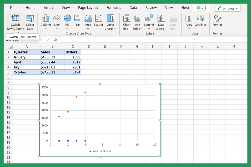
- Click the Scatter chart button.
- Click the Switch Row/Column button on the Chart Tools Layout tab.
Your data should now be displayed with the correct axis.
What Is an Excel Line Chart & What Does It Have To Do With X and Y Values?
A line chart is a graph that shows how data changes over time. Line charts are typically used to track changes in data over time, but they can also be used to compare data sets. Line charts can be created in Excel by selecting the Insert tab and then clicking on the Line chart button.
When you create a line chart, Excel will automatically put the variable on the x-axis and the dependent variable on the y-axis. You can switch the axes by clicking on the Switch Row button on the Chart Tools Layout tab.
It is important to pay attention to the scale of your data when you are creating line charts. The scale is the range of values that are shown on each axis. If one axis has a much larger scale than another, it can make your graph look distorted.
Switch Axes in Scatter Charts & Scatterplots
A scatter chart is a graph that shows how two data sets are related to each other. Scatter charts are typically used to show how two data sets are related to each other. Scatter charts can be created in Excel by selecting the Insert tab and then clicking on the Scatter chart button.
When you create a scatter chart, Excel will automatically put the variable on the x-axis and the dependent variable on the y-axis. You can switch the axes on the Scatter chart by clicking on the Switch Row button on the Chart Tool Layout tab.
Is A Scatterplot and Scatter Chart the Same Thing?
While both scatterplots and scatter charts can be used to show how two data sets are related to each other, scatter charts are typically used to show how two data sets are related to each other.
Scatterplots can be created in Excel by selecting the Insert tab and then clicking on the Scatterplot button. When you create a scatterplot, Excel will automatically put the variable on the x-axis and the dependent variable on the y-axis. You can switch the axes by clicking on the Switch Row/Column button on the Chart Tool Layout tab.
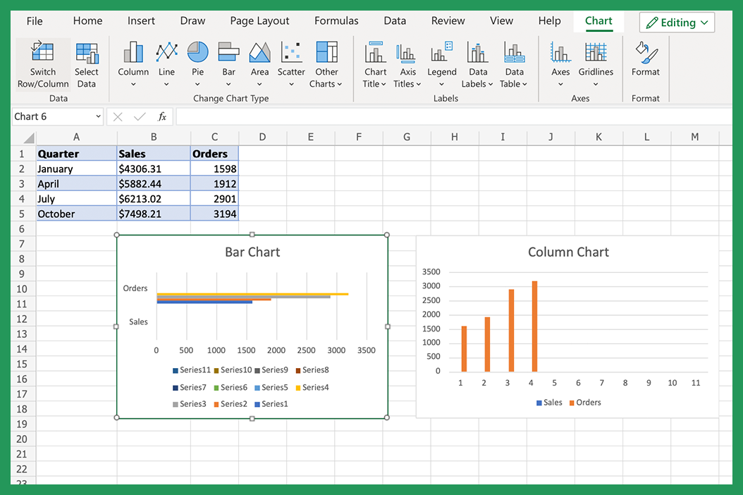
Switch Bar Graph & Column Chart's Axes (Built-In Charts)
The main difference between the two is that a bar graph is oriented horizontally while a column chart is oriented vertically. Other than that, both are used to compare worksheet data sets.
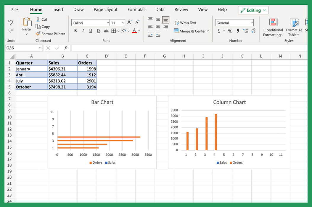
Bar graphs can be created in Excel by selecting the Insert tab and then clicking on the Bar graph button. When you create a bar graph, Excel will automatically put the variable on the x-axis and the dependent variable on the y-axis. You can switch the axes by clicking on the Switch Row button on the Chart Tool Layout tab.
Columns can be created in Excel by selecting the Insert tab and then clicking on the Column chart button. When you create a column chart, Excel will automatically put the variable on X and the dependent variable on the y-axis. You can switch the axes by clicking on the Switch Row or Column button on the Chart Tool Layout tab.
Switching X and Y Axis in Pie Charts
If you have a pie chart, you can switch the x and y axis by going to the "Chart Tool" tab on the ribbon and clicking "Layout." Then, click "Axis" and select "Primary Horizontal." This will switch x and y.
You can also change the order of the data values in your pie chart by rearranging your data before you switch the axis. To do this, go to the "Data" tab on the ribbon and click "Pivot Table." A new window will open. In this window, drag the field that you want to be your variable into the "Axis (X)" box and drag the field that you want to be your dependent variable into the "Values" box.
Once you have rearranged your data values, it's time to switch the axis. To do this, go to the "Chart Tool" tab on the ribbon and click "Layout." Then, click "Axis" and select "Secondary Axis." to switch rows.
Rearranging Your Data to Specify the Axis
To rearrange your data so that the dependent variable is first and the variable is second, you will need to use a function called "pivot." Pivot allows you to change the structure of your data without changing the original data itself. To use pivot, select the cell that contains your data set. Then, go to the "Data" tab on the ribbon and click "Pivot Table." A new window will open. In this window, drag the field that you want to be your variable that's independent into the "Axis (X)" box and drag the field that you want to be your dependent variable into the "Values" box.
Once you have rearranged your data set, it's time to switch the axis. To do this, go to the "Chart Tool" tab on the ribbon and click "Layout." Then, click "Axes" and select "Secondary Axis." This will switch x and y.
That's all there is to it! Switching the x and y axis is easy once you know how. Try it out with your own data sets and see how it can help you compare different types of information.
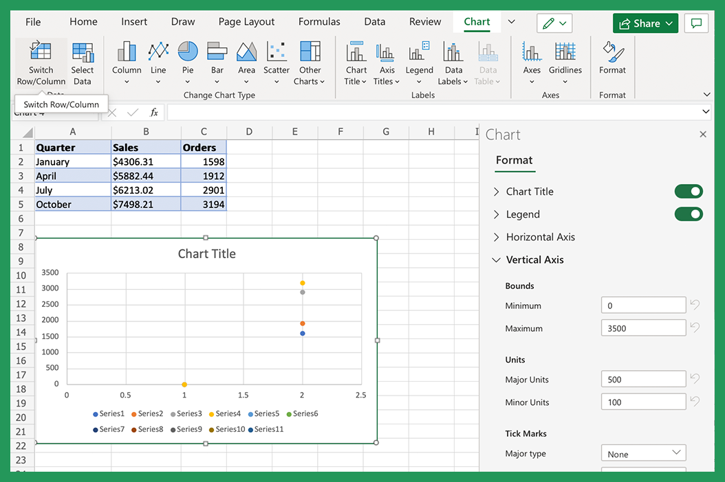
How to Select Data to Change the Y-Axis
It is often necessary in graphing to change the range or scale of numbers on the y-axis. This can be done in Excel when you select data that you want included, then going to the "Chart Tool" tab on the ribbon. Click "Layout" and then "Axis." From here, you can select the "Minimum" and "Maximum" values for your y-axis.
You can also change the scale of your y-axis by clicking on the "Logarithmic Scale" option. This will change the way it is displayed and can be helpful when you are working with large numbers.
When you are changing the scale of your y-axis, it is important to pay attention to the units of measurement. Make sure that the numbers on your axis are consistent with the rest of your worksheet. You can also select data source window to make these changes.
Summary & Overview for Excel Newbies
You can switch the x and y axis in Excel by rearranging your data and using the "Secondary Axis" option in the "Chart Tool" tab.
When you are working with chart axes, it is important to pay attention to the units of measurement and the scale of the data.
Switching the x and y axis can be a helpful way to compare different types of data. Try it out with your own data sets and see how it can help you understand your information better. Thanks for reading! We hope this was helpful.
What to Avoid When Switching the X and Y Axis
There are a few things to avoid when you are switching the x and y values manually in Excel. First, make sure that your values are arranged correctly. The variable should be in the first column and the dependent variable should be in the second column.
You should avoid using the "Switch Row/Column" button on the Chart Tool Layout tab. This will switch the x-axis and y-axis, but it will also switch the data in your cells. If you want to keep your spreadsheet intact, use the pivot function to rearrange your data before you switch the axes.
Conclusion
Switching the x and y axis in Excel is easy once you know how. Try it out with your own data sets and see how it can help you compare different types of information. Excel is an amazing way to store data, and showcase it in any way you want to. This does mean it can be quite tricky to get the hang of if you're a beginner. We hope this article has been helpful to you!
Do you have any questions about switching the x and y axis in Excel? Contact us and we'll be happy to help. And be sure to search or check back soon for more helpful tips and tricks. Thanks for reading!